Crack Surface Density Functional#

Before studying phase-field fracture simulation—which couples displacement (elasticity) and phase-field—it is recommended to first understand each problem independently. Here, we focus on the crack surface density functional alone, as described in Miehe et al.[1].

The aim of this functional is to provide a continuous representation of a discontinuous field. It should be noted that when the length scale parameter tends to 0, the continuous representation approximates the discontinuous case.

Note

Please view the examples related to the crack surface density functional in Phase-Field.

Variational approach#

The problem that needs to be solved is stationary and derives from an optimization principle.

The phase field is given by the minimizer of the crack surface density functional:

\[W[\phi] = \int_\Omega \left( \frac{1}{2l} \phi^2 + \frac{l}{2} |\nabla \phi|^2 \right) dV\]

The equilibrium equations can be recovered from the optimality condition \(\delta W = 0\).

Next, we calculate the variations of the functional by applying the Gateaux derivative:

\[\begin{split}\delta_\phi W & = \frac{d}{d \epsilon} W (\phi+\epsilon\delta_\phi) \bigg\rvert_{\epsilon=0} \\ & = \frac{d}{d \epsilon} \int \left( \frac{1}{2l}(\phi+\epsilon\delta_\phi)^2 + \frac{l}{2} |\nabla (\phi+\epsilon\delta_\phi)|^2 \right) dV \bigg\rvert_{\epsilon=0} \\ & = \int \left( \frac{1}{2l} 2(\phi+\epsilon\delta_\phi)\delta_\phi + \frac{l}{2} 2(\nabla (\phi+\epsilon\delta_\phi))\cdot \nabla \delta_\phi \right) dV \bigg\rvert_{\epsilon=0} \\ & = \int \left( \frac{1}{l} (\phi+\epsilon\delta_\phi)\delta_\phi + l (\nabla (\phi+\epsilon\delta_\phi))\cdot \nabla \delta_\phi \right) dV \bigg\rvert_{\epsilon=0} \\ & = \int \left( \frac{1}{l} \phi \delta_\phi + l \nabla \phi \cdot \nabla \delta_\phi \right) dV\end{split}\]

So, the weak form of the phase-field problem is given by:

\[\int_\Omega \left( \frac{1}{l} \phi \delta\phi + l \nabla\phi \cdot \nabla \delta \phi \right) dV = 0\]

The strong form is given by:

\[\frac{1}{l}\phi - l \nabla^2 \phi = 0\]

and

\[\nabla \phi \cdot \mathbf{n} = 0 \quad \text{on} \quad \partial \Omega\]

One dimension solution#

Consider a broken bar with length \(L\), as depicted in fig fig:bar_with_center_crack , featuring a crack positioned at its center.

For the one-dimensional scenario, the functional reads:

\[W_{1D}[\phi] = \int_\Omega \left( \frac{1}{2l} \phi^2 + \frac{l}{2} \phi'^2 \right) dx\]

subject to the boundary conditions\(\phi(0) = 1\), and \(\phi'(\pm A) = 0\).

The problem can be reduced to a simple ordinary differential equation, with boundary conditions \(\phi(0) = 1\), and \(\phi'(A) = 0\):

\[\frac{1}{l}\phi(x) + l \phi''(x) = 0\]

The solution to this equation is given by:

\[\phi(x) = e^{-|x|/l} + \frac{1}{e^{\frac{2a}{l}}+1} 2 \sinh \left( \frac{|x|}{l} \right)\]

\[\nabla \phi(x) = \frac{-\text{sign}(x)}{l} e^{-|x|/l} + \frac{1}{e^{\frac{2a}{l}} +1} \frac{\text{sign}(x)}{l} 2 \cosh\left(\frac{|x|}{l}\right)\]

Note

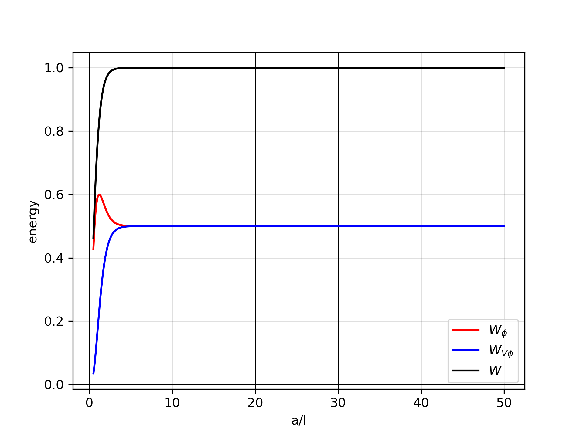
Note that Miehe et al.[1] considers an infinite domain (or infinite bar). Therefore, as \(a/l \rightarrow \infty\), the solution approaches that of Miehe—corresponding to an infinite bar when \(a \rightarrow \infty\), or equivalently, to \(l \rightarrow 0\) for a finite bar. In both cases, the solution presented in Miehe et al.[1] is recovered.

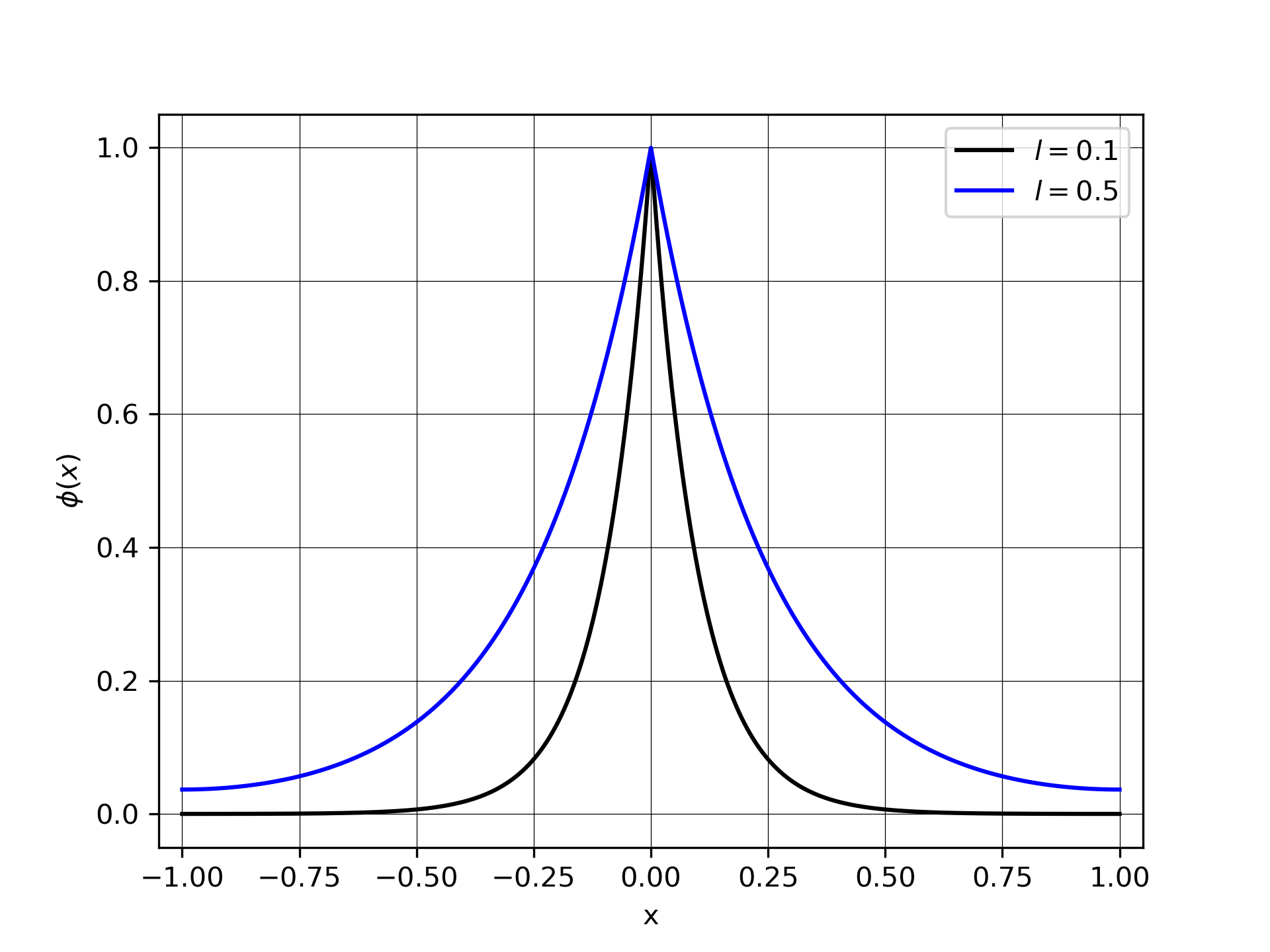
The phase field along the bar for two different length scales, \(l=1.0\) and \(l=0.5\), is shown in the following figure.

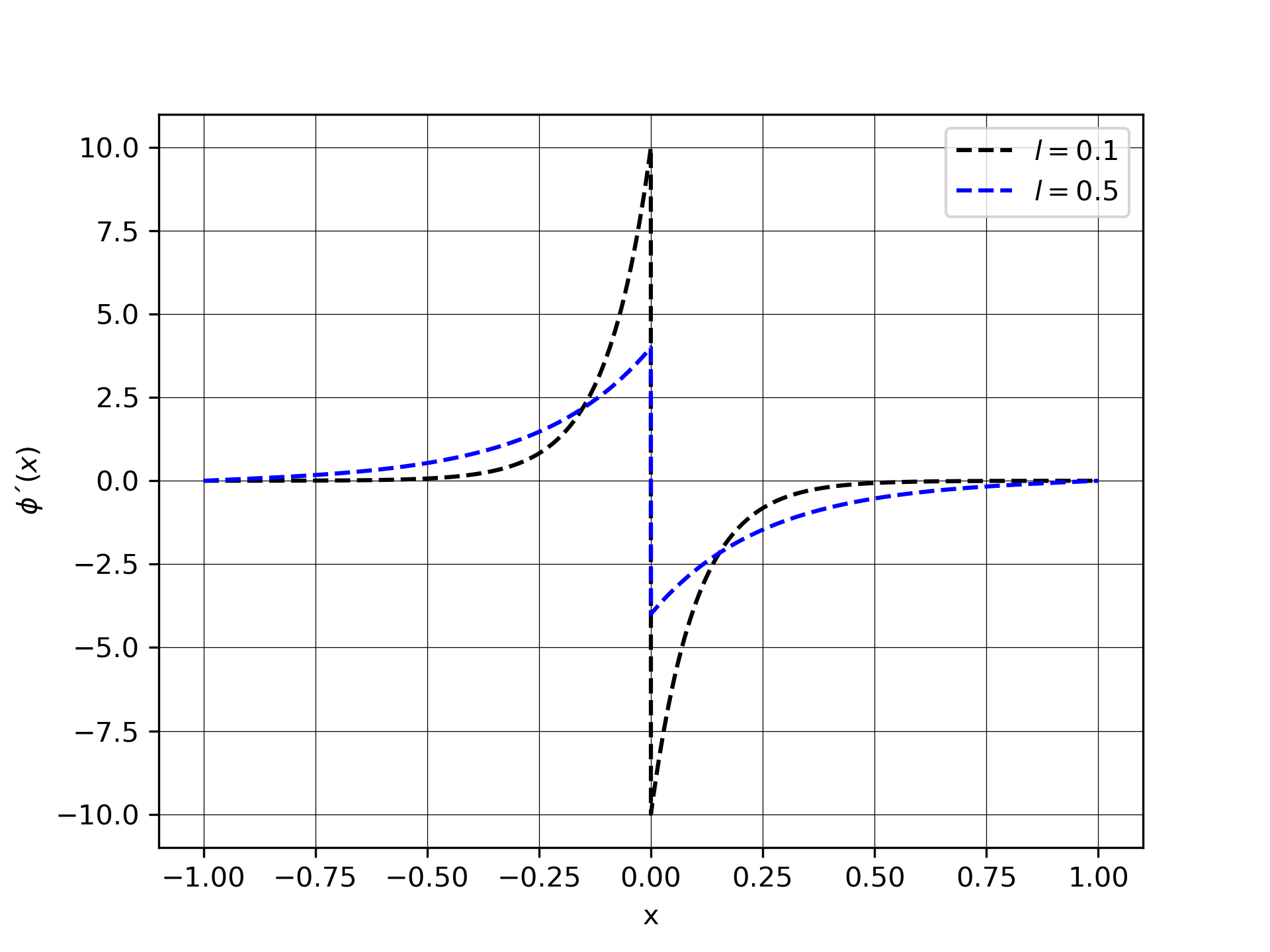
The corresponding gradients are also shown.

Energy#

With the obtained solution, it is possible to calculate the energy values of the bar. The energy functional can be written as:

\[W(\phi(x)) = \int_\Omega \left( \frac{1}{2l}\phi^2 + \frac{l}{2} \phi'^2 \right)dx\]

This energy can be separated into two contributions:

\[W_{\phi}(\phi(x)) = \int \frac{1}{2l}\phi(x)^2 dx\]

\[W_{\nabla \phi}(\phi(x)) = \int \frac{l}{2}\phi'(x)^2 dx\]

The total energy is then the sum of these contributions:

\[W(\phi(x)) = W_{\phi}(\phi(x)) + W_{\nabla \phi}(\phi(x))\]

Integrating over the one-dimensional domain, we find:

\[W_{\phi} = \frac{1}{2l} \int_{-a}^{a} \left[ e^{-|x|/l} + \frac{1}{e^{\frac{2a}{l}}+1} 2 \sinh \left( \frac{|x|}{l} \right) \right]^2 dx\]

\[W_{\nabla \phi}(\phi) = \frac{l}{2} \int_{-a}^{a} \left[ \frac{-\text{sign}(x)}{l} e^{-|x|/l} + \frac{1}{e^{\frac{2a}{l}} +1} \frac{\text{sign}(x)}{l} 2 \cosh\left(\frac{|x|}{l}\right) \right]^2 dx\]

Therefore, the total energy is given by:

\[W = \tanh \left( \frac{a}{l} \right)\]

\[W_{\phi} = \frac{1}{2} \tanh \left( \frac{a}{l} \right) + \frac{1}{2} \frac{a}{l} \left[ 1-\tanh^2 \left( \frac{a}{l} \right) \right]\]

\[W_{\nabla \phi} = \frac{1}{2} \tanh \left( \frac{a}{l} \right) - \frac{1}{2} \frac{a}{l} \left[ 1-\tanh^2 \left( \frac{a}{l} \right) \right]\]

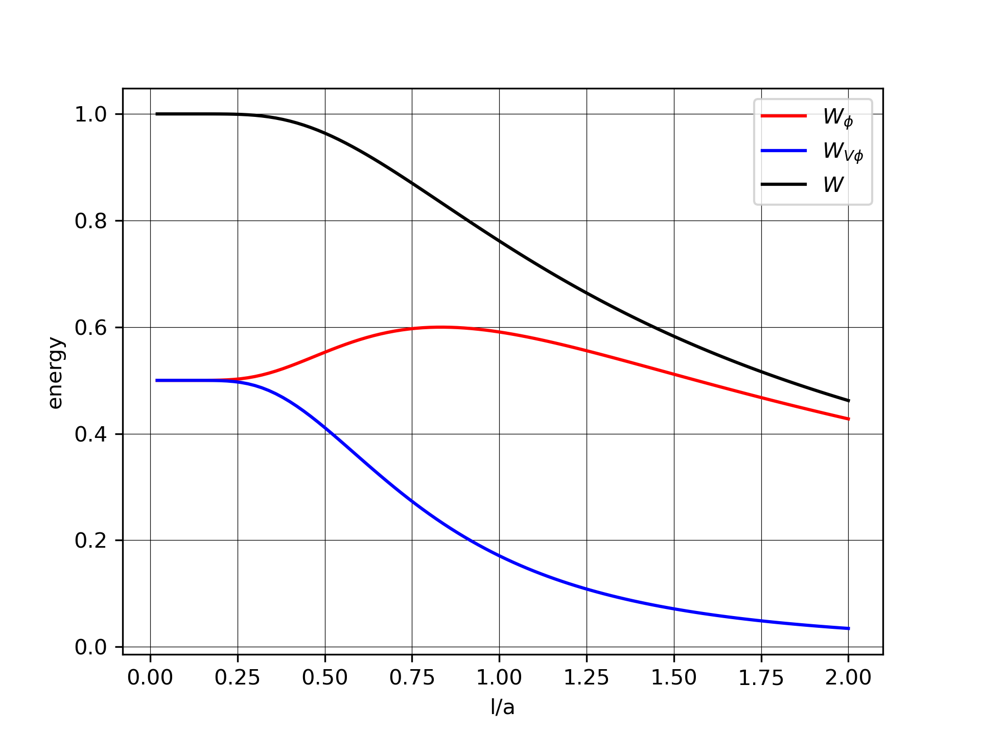
The following figure displays the energy of the bar for different values of the length scale \(l/a\):

Additionally, the figure shows the energy versus the \(a/l\) relation: