Free Energy: Allen-Cahn

In this example, we study the free energy potential of the Allen-Cahn equation. The model consists of a bar of length \(2a\) with boundary conditions at \(x=-a\) of \(\phi=-1\) and \(\phi=1\) at \(x=a\). The theoric framework is explained in (Allen Cahn).

#
#
#         *------------------------*
#  phi=-1 |           * (0,0)      | phi=1
#         *------------------------*
#
#         |<----a----->|<-----a---->|
#     |Y
#     |
#     *---X

The potential is the following:

\[W[\phi] = \int_\Omega \left( \frac{1}{l}f_{chem}(\phi) + \frac{l}{2} |\nabla \phi|^2 \right) dV\]

with

\[f_{chem}(\phi) = \frac{1}{4}(1-\phi^2)^2\]

as described in the theory section (Allen Cahn). The one-dimensional solution for an infinite domain is given by:

\[\phi(x) = \tanh\left(\frac{x}{\sqrt{2}l}\right)\]

In this case, the domain and the length scale parameter can be interpreted as an infinite domain (see the table values), as \(tanh\left(\frac{a}{\sqrt{2}a}\right)=1\) and \(tanh\left(\frac{-a}{\sqrt{2}a}\right)=-1\), so it is in concordance with the boundary conditions imposed.

Properties

	VALUE	UNITS
l	10.0	mm
a	50.0	mm

Import necessary libraries

import numpy as np
import matplotlib.pyplot as plt
import pyvista as pv
import dolfinx
import mpi4py
import os

Import from phasefieldx package

from phasefieldx.Element.Allen_Cahn.Input import Input
from phasefieldx.Element.Allen_Cahn.solver.solver_static import solve
from phasefieldx.Boundary.boundary_conditions import bc_phi, get_ds_bound_from_marker
from phasefieldx.PostProcessing.ReferenceResult import AllResults

Parameters definition

First, we define an input class, which contains all the parameters needed for the setup and results of the simulation.

The first term, \(l\), specifies the length scale parameter for the problem, with \(l = 10.0\).

The next two options, save_solution_xdmf and save_solution_vtu, determine the file format used to save the phase-field results (.xdmf or .vtu), which can then be visualized using tools like ParaView or pvista. Both parameters are boolean values (True or False). In this case, we set save_solution_vtu=True to save the phase-field results in .vtu format.

Lastly, results_folder_name specifies the name of the folder where all results and log information will be saved. If the folder does not exist, phasefieldx will create it. However, if the folder already exists, any previous data in it will be removed, and a new empty folder will be created in its place.

Data = Input(l=10.0,
             save_solution_xdmf=False,
             save_solution_vtu=True,
             result_folder_name="4000_free_energy")

Mesh Definition

A 2a mm x 1 mm rectangular mesh with quadrilateral elements is created using Dolfinx. The mesh is a structured grid with quadrilateral elements:

• divx, divy: Number of elements along the x and y axes.

• lx, ly: Physical domain dimensions in x and y.

a = 50.0
divx, divy = 100, 1
lx, ly = 100.0, 1.0

msh = dolfinx.mesh.create_rectangle(mpi4py.MPI.COMM_WORLD,
                                    [np.array([-a, -0.5]),
                                     np.array([a, 0.5])],
                                    [divx, divy],
                                    cell_type=dolfinx.mesh.CellType.quadrilateral)

Boundary Identification

Boundary conditions and forces are applied to specific regions of the domain:

• left: Identifies the \(y=-a\) boundary.

• right: Identifies the \(y=a\) boundary.

• fdim is the dimension of boundary facets (1D for a 2D mesh).

def left(x):
    return np.isclose(x[0], -a)

def right(x):
    return np.isclose(x[0], a)

fdim = msh.topology.dim - 1

Using the bottom and top functions, we locate the facets on the left and right sides of the mesh, where \(x = -a\) and \(x = a\), respectively. The locate_entities_boundary function returns an array of facet indices representing these identified boundary entities.

left_facet_marker = dolfinx.mesh.locate_entities_boundary(msh, fdim, left)
right_facet_marker = dolfinx.mesh.locate_entities_boundary(msh, fdim, right)

The get_ds_bound_from_marker function generates a measure for applying boundary conditions specifically to the facets identified by left_facet_marker and right_facet_marker, respectively. This measure is then assigned to ds_left and ds_right.

ds_left = get_ds_bound_from_marker(left_facet_marker, msh, fdim)
ds_right = get_ds_bound_from_marker(right_facet_marker, msh, fdim)

ds_list is an array that stores boundary condition measures along with names for each boundary, simplifying result-saving processes. Each entry in ds_list is formatted as [ds_, “name”], where ds_ represents the boundary condition measure, and “name” is a label used for saving. Here, ds_left and ds_right are labeled as “left” and “right”, respectively, to ensure clarity when saving results.

ds_list = np.array([
                   [ds_left, "left"],
                   [ds_right, "right"]
                   ])

Function Space Definition

Define function spaces for the phase-field using Lagrange elements of degree 1.

V_phi = dolfinx.fem.functionspace(msh, ("Lagrange", 1))

Boundary Condition Setup for Scalar Field \(\phi\)

We define and apply a Dirichlet boundary condition for the scalar field \(\phi\) on the left side of the mesh, setting \(phi = -1\) on this boundary and on the right side of the mesh \(phi = 1\) on this boundary. This setup is for a simple, static linear problem, meaning the boundary conditions and loading are constant and do not change throughout the simulation.

• bc_phi is a function that creates a Dirichlet boundary condition on a specified facet of the mesh for the scalar field \(\phi\).

• bcs_list_phi is a list that stores all the boundary conditions for \(\phi\), facilitating easy management and extension of conditions if needed.

• update_boundary_conditions and update_loading are set to None as they are unused in this static case with constant boundary conditions and loading.

bc_left = bc_phi(left_facet_marker, V_phi, fdim, value=-1.0)
bc_right = bc_phi(right_facet_marker, V_phi, fdim, value=1.0)
bcs_list_phi = [bc_left, bc_right]
update_boundary_conditions = None
update_loading = None

Solver Call for a Static Linear Problem

We define the parameters for a simple, static linear boundary value problem with a final time t = 1.0 and a time step Δt = 1.0. Although this setup includes time parameters, they are primarily used for structural consistency with a generic solver function and do not affect the result, as the problem is linear and time-independent.

Parameters:

• final_time: The end time for the simulation, set to 1.0.

• dt: The time step for the simulation, set to 1.0. In a static context, this only provides uniformity with dynamic cases but does not change the results.

• path: Optional path for saving results; set to None here to use the default.

• quadrature_degree: Defines the accuracy of numerical integration; set to 2 for this problem.

Function Call: The solve function is called with:

• Data: Simulation data and parameters.

• msh: Mesh of the domain.

• V_phi: Function space for phi.

• bcs_list_phi: List of boundary conditions.

• update_boundary_conditions, update_loading: Set to None as they are unused in this static problem.

• ds_list: Boundary measures for integration on specified boundaries.

• dt and final_time to define the static solution time window.

final_time = 1.0
dt = 1.0

solve(Data,
      msh,
      final_time,
      V_phi,
      bcs_list_phi,
      update_boundary_conditions,
      update_loading,
      ds_list,
      dt,
      path=None,
      quadrature_degree=2)

All specified files deleted successfully.
All specified folders and their contents deleted successfully.
All specified folders and their contents deleted successfully.

Load results

Once the simulation finishes, the results are loaded from the results folder. The AllResults class takes the folder path as an argument and stores all the results, including logs, energy, convergence, and DOF files. Note that it is possible to load results from other results folders to compare results. It is also possible to define a custom label and color to automate plot labels.

S = AllResults(Data.results_folder_name)
S.set_label('Simulation')
S.set_color('b')

Plot: phase-field \(\phi\)

The phase-field result saved in the .vtu file is shown. For this, the file is loaded using PyVista.

file_vtu = pv.read(os.path.join(Data.results_folder_name, "paraview-solutions_vtu", "phasefieldx_p0_000000.vtu"))
file_vtu.plot(scalars='phi', cpos='xy', show_scalar_bar=True, show_edges=False)

Static Scene

Interactive Scene

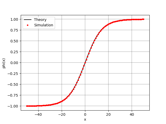
Plot: Phase-field along the x-axis

The phase-field value along the x-axis is plotted and compared with the analytic solution. The analytic solution is given by: \(\phi(x) = \tanh\left(\frac{x}{\sqrt{2}l}\right)\) Note: In this case, a = lx

xt = np.linspace(-a, a, 200)
phi_theory = np.tanh(xt / (Data.l * np.sqrt(2)))

fig, ax_phi = plt.subplots()

ax_phi.plot(xt, phi_theory, 'k-', label='Theory')
ax_phi.plot(file_vtu.points[:, 0], file_vtu['phi'], 'r.', label=S.label)

ax_phi.grid(color='k', linestyle='-', linewidth=0.3)
ax_phi.set_ylabel('phi(x)')
ax_phi.set_xlabel('x')
ax_phi.legend()

plt.show()

Energy values

The theoretical energy value is compared with the value calculated from the simulation.

energy_theory = np.sqrt(2) * np.tanh(a / (Data.l * np.sqrt(2))) - (1 / 3) * np.sqrt(2) * np.tanh(a / (Data.l * np.sqrt(2)))**3
energy_simulation = S.energy_files["total.energy"]["gamma"][0]
print(f"The theoretical energy is {energy_theory}")
print(f"The calculated numerical energy is {energy_simulation}")

The theoretical energy is 0.9428049702140735
The calculated numerical energy is 0.9429741358994296