Note
Go to the end to download the full example code.
Crack surface density functional#
In this example, we examine the boundary value problem related to the representation of a crack surface. This approach models the crack surface density functional, offering a continuous approximation of an otherwise discontinuous crack surface (Crack Surface Density Functional).
Due to the symmetry of the problem, we consider only the left half of the bar. A boundary condition is therefore applied at the left end of this half-bar, as shown in the diagrams below.
For a one-dimensional simulation, the boundary condition \(\phi=1\) is imposed at the left end of this segment.
#
#
#         x=0
#  phi= 1 *------------------------*
#
#         |<---------- lx --------->|
#     |Y
#     |
#     *---X
If two or three dimensions are considered, the boundary condition \(\\phi=1\) is applied to the left surface.
#         x=0
#         *------------------------*
#  phi= 1 |                        |
#         *------------------------*
#
#         |<---------- a --------->|
#     |Y
#     |
#     *---X
Three dimensions:
#           *------------------------*
#          /                        /|
#         *------------------------* |
#  phi= 1 |                        |/
#         *------------------------*
#
#         |<---------- a --------->|
#     |Y
#     |
#     *---X
#   Z/
Import necessary libraries#
import numpy as np
import matplotlib.pyplot as plt
import pyvista as pv
import dolfinx
import mpi4py
import os
Import from phasefieldx package#
from phasefieldx.Element.Phase_Field.Input import Input
from phasefieldx.Element.Phase_Field.solver.solver import solve
from phasefieldx.Boundary.boundary_conditions import bc_phi, get_ds_bound_from_marker
from phasefieldx.PostProcessing.ReferenceResult import AllResults
Parameters definition#
First, we define an input class, which contains all the parameters needed for the setup and results of the simulation.
The first term, \(l\), specifies the length scale parameter for the problem, with \(l = 4.0\).
The next two options, save_solution_xdmf and save_solution_vtu, determine the file format used to save the phase-field results (.xdmf or .vtu), which can then be visualized using tools like ParaView or pvista. Both parameters are boolean values (True or False). In this case, we set save_solution_vtu=True to save the phase-field results in .vtu format.
Lastly, results_folder_name specifies the name of the folder where all results and log information will be saved. If the folder does not exist, phasefieldx will create it. However, if the folder already exists, any previous data in it will be removed, and a new empty folder will be created in its place.
Data = Input(
    l=1.0,
    save_solution_xdmf=False,
    save_solution_vtu=True,
    results_folder_name="2000_General"
)
Mesh Definition#
We define the mesh parameters and set up a two-dimensional simulation. This setup supports various dimensions (‘1D’, ‘2D’, or ‘3D’) by creating a mesh that consists of either a line, rectangle, or box, depending on the selected dimension, with corresponding line, quadrilateral, or hexahedral elements.
divx, divy, and divz specify the number of divisions along the x, y, and z
axes, respectively. Here, divx=100, divy=1, and divz=1 are set to divide the x-axis primarily, as needed for a 2D or 1D mesh.
lx, ly, and lz define the physical dimensions of the domain in the x, y, and z
directions. In this example, we set lx=5.0, ly=1.0, and lz=1.0.
Specify the simulation dimension with the dimension variable (“1d”, “2d”, or “3d”). Here, we choose “2d”.
divx, divy, divz = 100, 1, 1
lx, ly, lz = 5.0, 1.0, 1.0
dimension = "2d"

# Mesh creation based on specified dimension
if dimension == "1d":
    # Creates a 1D mesh, which consists of a line divided into `divx` line elements,
    # extending from 0 to lx along the x-axis.
    msh = dolfinx.mesh.create_interval(
        mpi4py.MPI.COMM_WORLD,
        divx,
        np.array([0.0, lx])
    )

elif dimension == "2d":
    # Creates a 2D mesh, which consists of a rectangle covering [0, 0] to [lx, ly] with `divx`
    # divisions in x and `divy` divisions in y, using quadrilateral elements.
    msh = dolfinx.mesh.create_rectangle(
        mpi4py.MPI.COMM_WORLD,
        [np.array([0.0, 0.0]), np.array([lx, ly])],
        [divx, divy],
        cell_type=dolfinx.mesh.CellType.quadrilateral
    )

elif dimension == "3d":
    # Creates a 3D mesh, which consists of a box extending from [0, 0, 0] to [lx, ly, lz],
    # divided into `divx`, `divy`, and `divz` parts along the x, y, and z axes, respectively,
    # with hexahedral elements.
    msh = dolfinx.mesh.create_box(
        mpi4py.MPI.COMM_WORLD,
        [np.array([0.0, 0.0, 0.0]), np.array([lx, ly, lz])],
        [divx, divy, divz],
        cell_type=dolfinx.mesh.CellType.hexahedron
    )
Left Boundary Identification#
This function identifies points on the left side of the domain where the boundary condition will be applied. Specifically, it returns True for points where x=0, and False otherwise. This allows us to selectively apply boundary conditions only to this part of the mesh.
def left(x):
    return np.equal(x[0], 0)
fdim represents the dimension of the boundary facets on the mesh, which is one less than the mesh’s overall dimensionality (msh.topology.dim). For example, if the mesh is 2D, fdim will be 1, representing 1D boundary edges.
fdim = msh.topology.dim - 1
Using the left function, we locate the facets on the left side of the mesh where x=0. The locate_entities_boundary function returns an array of facet indices that represent the identified boundary entities.
left_facet_marker = dolfinx.mesh.locate_entities_boundary(msh, fdim, left)
get_ds_bound_from_marker is a function that generates a measure for integrating boundary conditions specifically on the facets identified by left_facet_marker. This measure is assigned to ds_left and will be used for applying boundary conditions on the left side.
ds_left = get_ds_bound_from_marker(left_facet_marker, msh, fdim)
ds_list is an array that stores boundary condition measures and associated names for each boundary to facilitate result-saving processes. Each entry in ds_list is an array in the form [ds_, “name”], where ds_ is the boundary condition measure, and “name” is a label for saving purposes. Here, ds_left is labeled as “left” for clarity when saving results.
ds_list = np.array([
                   [ds_left, "left"],
                   ])
Function Space Definition#
Define function spaces for the phase-field using Lagrange elements of degree 1.
V_phi = dolfinx.fem.functionspace(msh, ("Lagrange", 1))
V_gradient_phi = dolfinx.fem.functionspace(msh, ("Lagrange", 1, (msh.geometry.dim, )))
Boundary Condition Setup for Scalar Field \(\phi\)#
We define and apply a Dirichlet boundary condition for the scalar field \(\phi\) on the left side of the mesh, setting \(phi = 1\) on this boundary. This setup is for a simple, static linear problem, meaning the boundary conditions and loading are constant and do not change throughout the simulation.
bc_phi is a function that creates a Dirichlet boundary condition on a specified facet of the mesh for the scalar field \(\phi\).
bcs_list_phi is a list that stores all the boundary conditions for \(\phi\), facilitating easy management and extension of conditions if needed.
update_boundary_conditions and update_loading are set to None as they are unused in this static case with constant boundary conditions and loading.
bc_left = bc_phi(left_facet_marker, V_phi, fdim, value=1.0)
bcs_list_phi = [bc_left]
update_boundary_conditions = None
update_loading = None
Solver Call for a Static Linear Problem#
We define the parameters for a simple, static linear boundary value problem with a final time t = 1.0 and a time step Δt = 1.0. Although this setup includes time parameters, they are primarily used for structural consistency with a generic solver function and do not affect the result, as the problem is linear and time-independent.
Parameters:
final_time: The end time for the simulation, set to 1.0.
dt: The time step for the simulation, set to 1.0. In a static context, this only provides uniformity with dynamic cases but does not change the results.
path: Optional path for saving results; set to None here to use the default.
quadrature_degree: Defines the accuracy of numerical integration; set to 2 for this problem.
Function Call: The solve function is called with:
Data: Simulation data and parameters.
msh: Mesh of the domain.
V_phi: Function space for phi.
bcs_list_phi: List of boundary conditions.
update_boundary_conditions, update_loading: Set to None as they are unused in this static problem.
ds_list: Boundary measures for integration on specified boundaries.
dt and final_time to define the static solution time window.
final_time = 1.0
dt = 1.0

solve(Data,
      msh,
      final_time,
      V_phi,
      bcs_list_phi,
      update_boundary_conditions,
      update_loading,
      ds_list,
      dt,
      path=None,
      quadrature_degree=2,
      V_gradient_Φ=V_gradient_phi)
All specified files deleted successfully.
All specified folders and their contents deleted successfully.
All specified folders and their contents deleted successfully.
Load results#
Once the simulation finishes, the results are loaded from the results folder. The AllResults class takes the folder path as an argument and stores all the results, including logs, energy, convergence, and DOF files. Note that it is possible to load results from other results folders to compare results. It is also possible to define a custom label and color to automate plot labels.
S = AllResults(Data.results_folder_name)
S.set_label('Simulation')
S.set_color('b')
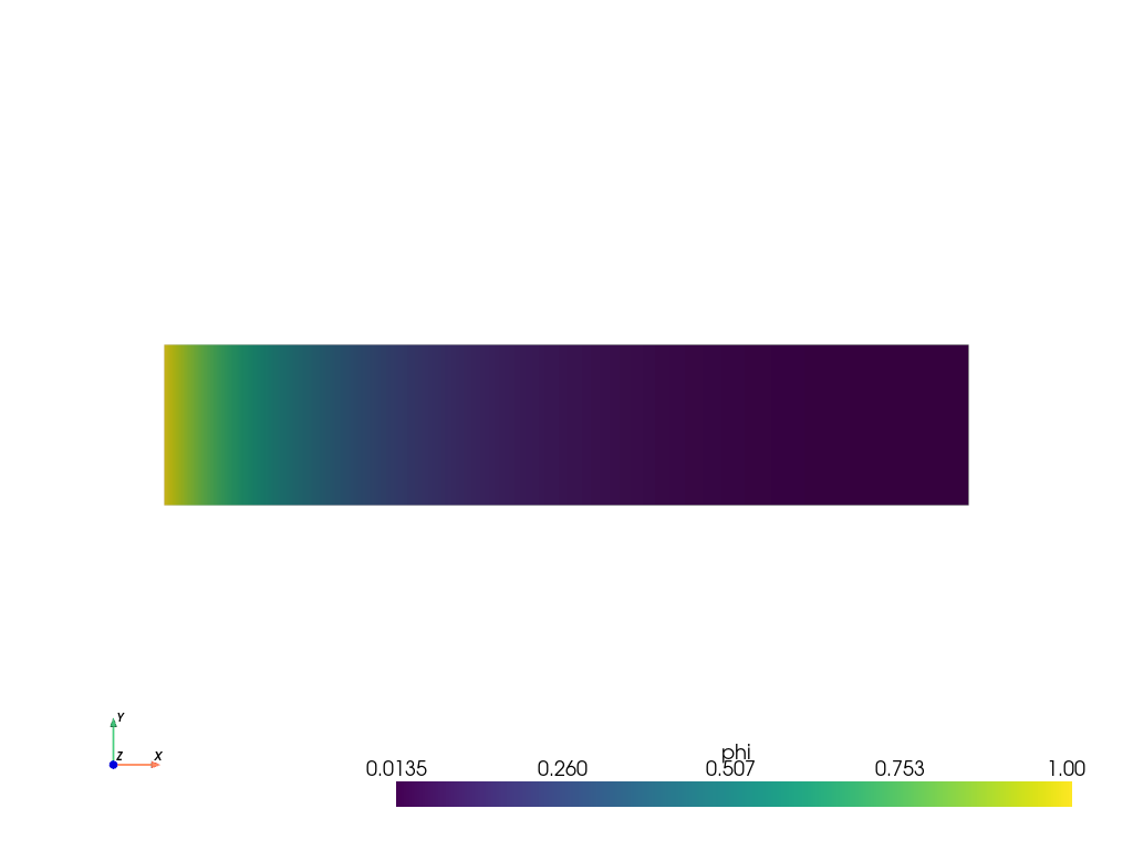
Plot: phase-field \(\phi\)#
The phase-field result saved in the .vtu file is shown. For this, the file is loaded using PyVista.
file_vtu = pv.read(os.path.join(Data.results_folder_name, "paraview-solutions_vtu", "phasefieldx000000.pvtu"))
file_vtu.plot(scalars='phi', cpos='xy', show_scalar_bar=True, show_edges=False)
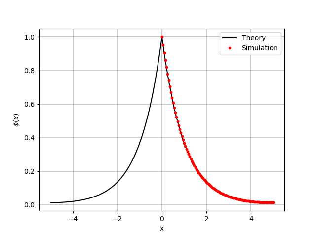
Plot: Phase-field along the x-axis#
The phase-field value along the x-axis is plotted and compared with the analytic solution. The analytic solution is given by: $phi(x) = e^{-|x|/l} + frac{1}{e^{frac{2a}{l}}+1} 2 sinh left(frac{|x|}{l} right)$ Note: in this case a = lx
xt = np.linspace(-lx, lx, 1000)
phi_theory = np.exp(-abs(xt) / Data.l) + 1 / (np.exp(2 * lx / Data.l) + 1) * 2 * np.sinh(np.abs(xt) / Data.l)

fig, ax_phi = plt.subplots()

ax_phi.plot(xt, phi_theory, 'k-', label='Theory')
ax_phi.plot(file_vtu.points[:, 0], file_vtu['phi'], 'r.', label=S.label)

ax_phi.grid(color='k', linestyle='-', linewidth=0.3)
ax_phi.set_ylabel('$\\phi(x)$')
ax_phi.set_xlabel('x')
ax_phi.legend()
<matplotlib.legend.Legend object at 0x74432baa2a70>
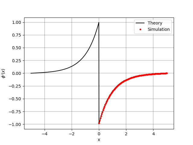
Plot: Phase-field gradient along the x-axis#
The phase-field gradient along the x-axis is plotted and compared with the analytic solution. The analytic solution is given by: $phi’(x) = -frac{1}{l} e^{-|x|/l} + frac{1}{e^{frac{2a}{l}}+1} frac{2}{l} coshleft(frac{|x|}{l}right)$ Note: in this case a = lx
one_div_exp2adivl_one = 1 / (np.exp(2 * lx / Data.l) + 1)
phi_gradient_theory = -np.sign(xt) / Data.l * np.exp(-abs(xt) / Data.l) + one_div_exp2adivl_one * np.sign(xt) / Data.l * 2 * np.cosh(np.abs(xt) / Data.l)

fig, ax_phi = plt.subplots()

ax_phi.plot(xt, phi_gradient_theory, 'k-', label='Theory')
ax_phi.plot(file_vtu.points[:, 0], file_vtu['gradient_phi'][:, 0], 'r.', label=S.label)

ax_phi.grid(color='k', linestyle='-', linewidth=0.3)
ax_phi.set_ylabel('$\\phi\'(x)$')
ax_phi.set_xlabel('x')
ax_phi.legend()
<matplotlib.legend.Legend object at 0x744320ce92d0>
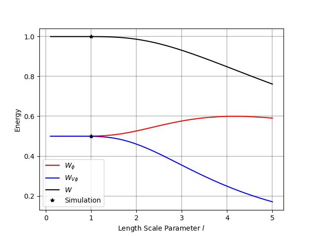
Plot: Energy Values Comparison#
In this section, we compare the energy values obtained from the simulation with their corresponding analytic expressions.
The energy components are calculated for the scalar field phi and its gradient. We compare the following energy terms:
W_phi: The energy associated with the scalar field phi. $W_{phi} = frac{1}{2l} int_{-a}^{a} left[ e^{-|x|/l} + frac{1}{e^{frac{2a}{l}}+1} 2 sinh left( frac{|x|}{l} right) right]^2 dx$
W_gradphi: The energy associated with the gradient of the scalar field. $W_{nabla phi}(phi) = frac{l}{2} int_{-a}^{a} left[ frac{-text{sign}(x)}{l} e^{-|x|/l} + frac{1}{e^{frac{2a}{l}} +1} frac{text{sign}(x)}{l} 2 coshleft(frac{|x|}{l}right) right]^2 dx$
W: The total energy, which includes contributions from both the field and its gradient. \(W = \tanh \left( \frac{a}{l} \right)\)
Theoretical expressions are computed for these energies as functions of the length scale parameter l. Additionally, energy values from the simulation are overlaid on the theoretical curve for comparison.
l_array = np.linspace(0.1, lx, 100)  # Create an array of length scale values
a_div_l = lx / l_array  # Compute the ratio of `lx` to the length scale
tanh_a_div_l = np.tanh(a_div_l)  # Compute the hyperbolic tangent of the ratio
Compute the theoretical energy for the scalar field phi The expression represents the energy of phi based on the length scale parameter l.
W_phi = 0.5 * tanh_a_div_l + 0.5 * a_div_l * (1.0 - tanh_a_div_l**2)
Compute the theoretical energy for the gradient of phi This energy is based on the gradient of phi and the length scale parameter l.
W_gradphi = 0.5 * tanh_a_div_l - 0.5 * a_div_l * (1.0 - tanh_a_div_l**2)
Compute the total theoretical energy This energy is related to the hyperbolic tangent of the ratio a/l.
W = np.tanh(a_div_l)
Plotting Energy Comparison#
The following plot compares the theoretical energy values (W_phi, W_gradphi, and W) with the energy values obtained from the simulation for various length scale parameters l. The simulation results are plotted as points on top of the theoretical curves to assess the agreement between theory and the computed values.
fig, energy = plt.subplots()  # Create a figure for plotting energy

energy.plot(l_array, W_phi, 'r-', label=r'$W_{\phi}$')  # Energy for `phi`
energy.plot(l_array, W_gradphi, 'b-', label=r'$W_{V \phi}$')  # Energy for gradient of `phi`
energy.plot(l_array, W, 'k-', label='$W$')  # Total energy

energy.plot(Data.l, 2 * S.energy_files['total.energy']["gamma_phi"][0], 'k*', label=S.label)
energy.plot(Data.l, 2 * S.energy_files['total.energy']["gamma_gradphi"][0], 'k*')
energy.plot(Data.l, 2 * S.energy_files['total.energy']["gamma"][0], 'k*')

energy.set_xlabel(r'Length Scale Parameter $l$')
energy.set_ylabel(r'Energy')
energy.grid(color='k', linestyle='-', linewidth=0.3)
energy.legend()

plt.show()
Total running time of the script: (0 minutes 1.488 seconds)