Note
Go to the end to download the full example code.
Fatigue: Single edge notched tension test#
In this study, a phase-field fatigue simulation is analyzed. The theoretical foundation of this model is presented in (Phase-field fracture). Specifically, a cyclic displacement is applied to a single-edge notched tension test, following the approach described by [Carrara]. The simulation adopts an isotropic formulation.
The model consists of a square plate with a notch located midway along the left edge, extending horizontally toward the center, as illustrated in the figure below. The bottom edge of the plate is fixed in all directions, while the top edge is free to slide vertically. A cyclic vertical displacement is applied to the top edge. The geometry and boundary conditions are clearly shown in the accompanying figure. The model is discretized using triangular finite elements, with refined mesh resolution (element size \(h\)) in regions where crack evolution is anticipated. The element size \(h\) must be sufficiently small to minimize mesh dependency.
A cyclic tensile test is performed under symmetric cyclic loading, with a displacement amplitude of \(\Delta u = 4 \times 10^{-3} mm\). The results are presented as fatigue life curves, showing the accumulation of the fatigue history variable \(\bar{\alpha}\) as a function of the number of cycles \(N\).
#                           /\
#                           ||
#            *----------*  ---- u
#            |          |   ||
#            | a=0.5    |   \/
#            |---       |
#            |          |
#            |          |
#            *----------*
#            /_\/_\/_\/_\
#     |Y    /////////////
#     |
#      ---X
#  Z /
Material Properties#
The material properties, length scale parameter, and fatigue parameter are summarized in the table below:
VALUE |
UNITS |
|
|---|---|---|
E |
210 |
kN/mm2 |
nu |
0.3 |
[-] |
Gc |
0.0027 |
kN/mm |
l |
0.004 |
mm |
alpha_n |
0.05625 |
kN/mm2 |

A framework to model the fatigue behavior of brittle materials based on a variational phase-field approach. P. Carrara, M. Ambati, R. Alessi, L. De Lorenzis. https://doi.org/10.1016/j.cma.2019.112731.
Import necessary libraries#
import numpy as np
import matplotlib.pyplot as plt
import pyvista as pv
import dolfinx
import mpi4py
import petsc4py
import os
Import from phasefieldx package#
from phasefieldx.Element.Phase_Field_Fracture.Input import Input
from phasefieldx.Element.Phase_Field_Fracture.solver.solver import solve
from phasefieldx.Boundary.boundary_conditions import bc_xy, bc_y, get_ds_bound_from_marker
from phasefieldx.PostProcessing.ReferenceResult import AllResults
Define Simulation Parameters#
Data is an input object containing essential parameters for simulation setup and result storage:
E: Young’s modulus, set to 210 \(kN/mm^2\).
nu: Poisson’s ratio, set to 0.3.
Gc: Critical energy release rate, set to 0.0027 \(kN/mm\).
l: Length scale parameter, set to 0.004 \(mm\).
degradation: Specifies the degradation type. Options are “isotropic” or “anisotropic”.
split_energy: Controls how the energy is split; options include “no” (default), “spectral,” or “deviatoric.”
degradation_function: Specifies the degradation function; here, it is “quadratic.”
irreversibility: Determines the irreversibility criterion; in this case, set to “miehe.”
fatigue: Enables fatigue simulation when set to True.
fatigue_degradation_function: Defines the function for fatigue degradation, set to “asymptotic.”
fatigue_val: Fatigue parameter value, set to \(0.05625\).
k: Stiffness penalty parameter, set to 0.0.
min_stagger_iter: Minimum number of staggered iterations, set to 2.
max_stagger_iter: Maximum number of staggered iterations, set to 500.
stagger_error_tol: Error tolerance for staggered iterations, set to 1e-8.
save_solution_xdmf and save_solution_vtu: Specify the file formats to save displacement results. In this case, results are saved as .vtu files.
results_folder_name: Name of the folder for saving results. If it exists, it will be replaced with a new empty folder.
Data = Input(E=210.0,    # young modulus
             nu=0.3,     # poisson
             Gc=0.0027,  # critical energy release rate
             l=0.004,    # lenght scale parameter
             degradation="isotropic",  # "isotropic" "anisotropic"
             split_energy="no",        # "spectral" "deviatoric"
             degradation_function="quadratic",
             irreversibility="miehe",  # "miehe"
             fatigue=True,
             fatigue_degradation_function="asymptotic",
             fatigue_val=0.05625,
             k=0.0,
             save_solution_xdmf=False,
             save_solution_vtu=True,
             results_folder_name="1800_Fatigue_Single_Edge_Notched_Tension_Test")
Mesh Definition#
The mesh is generated using Gmsh and saved as a ‘mesh.msh’ file. For more details on how to create the mesh, refer to the Examples gmsh “.geo” files examples.
msh_file = os.path.join("mesh", "mesh.msh")  # Path to the mesh file
gdim = 2                                     # Geometric dimension of the mesh
gmsh_model_rank = 0                          # Rank of the Gmsh model in a parallel setting
mesh_comm = mpi4py.MPI.COMM_WORLD            # MPI communicator for parallel computation
The mesh, cell markers, and facet markers are extracted from the ‘mesh.msh’ file using the read_from_msh function.
mesh_data = dolfinx.io.gmsh.read_from_msh(msh_file, mesh_comm, gmsh_model_rank, gdim)
msh = mesh_data.mesh
cell_markers = mesh_data.cell_tags
facet_markers = mesh_data.facet_tags

fdim = msh.topology.dim - 1 # Dimension of the mesh facets
Facets defined in the .geo file used to generate the ‘mesh.msh’ file are identified here. Each marker variable corresponds to a specific region on the specimen:
bottom_facet_marker: Refers to the bottom part of the specimen.
top_facet_marker: Refers to the top part of the specimen.
right_facet_marker: Refers to the right side of the specimen.
left_facet_marker: Refers to the left side of the specimen.
bottom_facet_marker = facet_markers.find(9)
top_facet_marker = facet_markers.find(10)
right_facet_marker = facet_markers.find(11)
left_facet_marker = facet_markers.find(12)
The get_ds_bound_from_marker function creates measures for applying boundary conditions on specific facets. These measures are generated for:
bottom_facet_marker → Stored in ds_bottom
top_facet_marker → Stored in ds_top
right_facet_marker → Stored in ds_right
left_facet_marker → Stored in ds_left
ds_bottom = get_ds_bound_from_marker(bottom_facet_marker, msh, fdim)
ds_top = get_ds_bound_from_marker(top_facet_marker, msh, fdim)
ds_right = get_ds_bound_from_marker(right_facet_marker, msh, fdim)
ds_left = get_ds_bound_from_marker(left_facet_marker, msh, fdim)
ds_list is an array that organizes boundary condition measures alongside descriptive names. Each entry in ds_list consists of two elements:
A measure (e.g., ds_bottom)
A corresponding name (e.g., “bottom”)
This structure simplifies the process of saving results by associating each boundary condition measure with a clear label. For instance:
ds_bottom is labeled as “bottom”.
ds_top is labeled as “top”.
ds_list = np.array([
                   [ds_bottom, "bottom"],
                   [ds_top, "top"]
                   ])
Function Space Definition#
Define function spaces for displacement and phase-field using Lagrange elements.
V_u = dolfinx.fem.functionspace(msh, ("Lagrange", 1, (msh.geometry.dim, )))
V_phi = dolfinx.fem.functionspace(msh, ("Lagrange", 1))
Boundary Conditions#
Dirichlet boundary conditions are defined as follows:
bc_bottom: Constrains both x and y displacements to 0 on the bottom boundary,
ensuring that the bottom edge is fixed. - bc_top: The vertical displacement on the top boundary is updated dynamically to impose the cyclic load.
The bcs_list_u variable is a list containing all boundary conditions for the displacement field, \(\boldsymbol{u}\). This structure simplifies the management of multiple boundary conditions and allows for easy expansion if additional conditions need to be applied.
bc_bottom = bc_xy(bottom_facet_marker, V_u, fdim)
bc_top = bc_y(top_facet_marker, V_u, fdim)
bcs_list_u = [bc_top, bc_bottom]
bcs_list_u_names = ["top", "bottom"]
Definition of the Cyclic Load#
The cyclic load is applied by updating the boundary condition at the top of the specimen. The cyclic load follows the form $ frac{2}{pi} A arcsin[sin(omega t)] $. where:
\(A = 0.002 \, \text{mm}\): Amplitude of the load.
\(f = \frac{1}{8}\): Frequency of the load in Hz.
\(\omega = 2 \pi f \): Angular frequency.
This periodic loading is imposed on the top boundary to simulate the desired cyclic behavior.
amplitude = 0.002
f = 1 / 8
w = 2 * np.pi * f
Function: update_boundary_conditions#
The update_boundary_conditions function dynamically modifies the boundary conditions at each time step, enabling the application of a cyclic load for quasi-static analysis. This function ensures that the displacement boundary condition evolves according to the prescribed cyclic loading function.
Parameters:
bcs: A list of boundary conditions, where each entry corresponds to a specific facet of the mesh.
For this implementation, bcs[0] refers to the top boundary condition. - time: A scalar representing the current time step in the simulation.
Inside the function:
val is computed based on the cyclic load formula: \(\text{val} = \frac{2}{\pi} \cdot \text{amplitude} \cdot \arcsin(\sin(\omega \cdot \text{time}))\)
where:
amplitude defines the maximum displacement of the cyclic load.
w (omega) is the angular frequency, given by ( omega = 2 pi f ), where ( f ) is the frequency.
The computed val represents the y-displacement applied to the boundary at the current time step.
This value is dynamically updated in bcs[0].g.value[…] to apply the displacement to the top boundary.
Returns:
A tuple (0, val, 0), where:
The first element is 0 (indicating no x-displacement).
The second element is val, the calculated y-displacement.
The third element is 0 (indicating no z-displacement, as this is a 2D simulation).
The function enables controlled cyclic loading during the simulation, facilitating the study of fatigue and quasi-static response under varying boundary conditions.
def update_boundary_conditions(bcs, time):
    val = 2 / np.pi * amplitude * np.arcsin(np.sin(w * time))
    bcs[0].g.value[...] = petsc4py.PETSc.ScalarType(val)
    return 0, val, 0

T_list_u = None
update_loading = None
Boundary Conditions for the Phase Field#
No boundary conditions are applied to the phase-field variable in this simulation.
bcs_list_phi = []
Solver Call for a Fatigue Problem#
This section defines the parameters and calls the solver for a phase-field fatigue problem.
Key Points:
The cyclic load and time parameters are synchronized to ensure 8 time steps are completed per cycle.
The solver function handles displacement updates and loading evolution for the quasi-static analysis.
Parameters:
dt: The time step for the simulation, set to 1.0.
final_time: The total simulation time, computed as ( 8 cdot 200 + 1 ), ensuring
sufficient steps for the cyclic loading behavior. - path: Optional parameter for specifying the results folder; set to None here to use the default location. - quadrature_degree: (Defined elsewhere) Specifies the accuracy of numerical integration during the computation. For this problem, it is set to 2.
Function Call: The solve function is invoked with the following arguments:
Data: Contains simulation parameters and configurations.
msh: The mesh of the domain.
final_time: The total simulation time.
V_u: Function space for the displacement field, \(\boldsymbol{u}\).
V_phi: Function space for the phase field, \(\phi\).
bcs_list_u: List of Dirichlet boundary conditions for the displacement field.
bcs_list_phi: List of boundary conditions for the phase field (empty in this case).
update_boundary_conditions: Function to dynamically update the displacement boundary conditions.
f: The body force applied to the domain (if any).
T_list_u: Time-dependent loading parameters for the displacement field.
update_loading: Function to update loading parameters for the quasi-static analysis.
ds_list: Boundary measures for integration over specified domain boundaries.
dt: The simulation time step.
path: Directory for saving simulation results (if specified).
This solver setup ensures a consistent and robust framework for solving the static linear problem while accommodating the cyclic loading behavior.
dt = 1.0
final_time = 8 * 200 + 1
Uncomment the following lines to run the solver with the specified parameters.
# solve(Data,
#       msh,
#       final_time,
#       V_u,
#       V_phi,
#       bcs_list_u,
#       bcs_list_phi,
#       update_boundary_conditions,
#       f,
#       T_list_u,
#       update_loading,
#       ds_list,
#       dt,
#       path=None,
#       bcs_list_u_names=bcs_list_u_names,
#       min_stagger_iter=2,
#       max_stagger_iter=500,
#       stagger_error_tol=1e-8)
Load results#
Once the simulation finishes, the results are loaded from the results folder. The AllResults class takes the folder path as an argument and stores all the results, including logs, energy, convergence, and DOF files. Note that it is possible to load results from other results folders to compare results. It is also possible to define a custom label and color to automate plot labels.
S = AllResults(Data.results_folder_name)
S.set_label('Simulation')
S.set_color('b')

cycles = S.dof_files["top.dof"]["#step"] * f
displacement = S.dof_files["top.dof"]["Uy"]
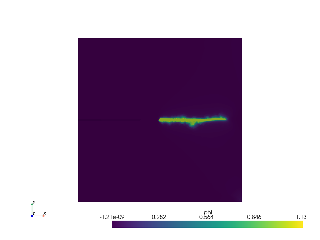
Plot: phase-field \(\phi\)#
The phase-field result saved in the .vtu file is shown. For this, the file is loaded using PyVista.
file_vtu = pv.read(os.path.join(Data.results_folder_name, "paraview-solutions_vtu", "phasefieldx_p0_001600.vtu"))

file_vtu.plot(scalars='phi', cpos='xy', show_scalar_bar=True, show_edges=False)
Plot: displacement \(\boldsymbol u\)#
The displacements results saved in the .vtu file are shown. For this, the file is loaded using PyVista.
file_vtu = pv.read(os.path.join(Data.results_folder_name, "paraview-solutions_vtu", "phasefieldx_p0_001600.vtu"))
file_vtu.plot(scalars='u', cpos='xy', show_scalar_bar=True, show_edges=False)

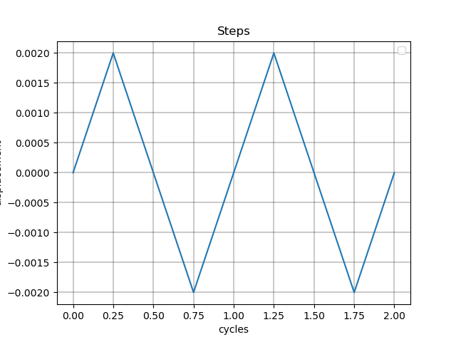
Plot: Cycles vs. Displacement#
This plot visualizes the relationship between cycles and displacement, focusing specifically on the first two cycles of the simulation.
fig, ax = plt.subplots()
ax.plot(cycles[0:2 * 8 + 1], S.dof_files["top.dof"]["Uy"][0:2 * 8 + 1], '-')
ax.grid(color='k', linestyle='-', linewidth=0.3)
ax.set_xlabel('cycles')
ax.set_ylabel('displacement')
ax.set_title('Steps')
ax.legend()
/home/docs/checkouts/readthedocs.org/user_builds/phasefieldx/checkouts/stable/examples/Fatigue/plot_1800.py:395: UserWarning: No artists with labels found to put in legend.  Note that artists whose label start with an underscore are ignored when legend() is called with no argument.
  ax.legend()

<matplotlib.legend.Legend object at 0x744320e4f0a0>
Plot: Cycles vs. Normalized \(\bar{\alpha}\) (for 3 cycles)#
This plot shows the evolution of the normalized fatigue history variable \(\bar{\alpha}\) as a function of the number of cycles, specifically for the first 3 complete cycles of the simulation.
The variable \(\bar{\alpha}\) represents the accumulation of fatigue damage, and in this plot, it is normalized by dividing the accumulated fatigue value by the maximum value over the first 3 cycles. This ensures that the fatigue history is scaled between 0 and 1, making it easier to compare the relative damage accumulation over the cycles.
The x-axis represents the number of cycles, up to 3 complete cycles (as indicated by cycles[:3 * 8]).
The y-axis represents the normalized fatigue history variable \(\bar{\alpha}\), scaled by the maximum value of \(\alpha\) accumulated over the first 3 cycles (aux2).
This plot is useful for analyzing the progression of fatigue accumulation over the first few cycles of loading.
fig, ax_alpha = plt.subplots()

aux2 = max(S.energy_files["total.energy"]["alpha_acum"][:3 * 8])
ax_alpha.plot(cycles[:3 * 8], S.energy_files["total.energy"]["alpha_acum"][:3 * 8] / aux2, 'r-', linewidth=2.0, label=r'$\bar{\alpha}$')
ax_alpha.grid(color='k', linestyle='-', linewidth=0.3)
ax_alpha.set_xlabel('cycles')
ax_alpha.set_ylabel(r'$\bar{\alpha}$')
ax_alpha.set_title(r'$\bar{\alpha}$ vs. number of cycles')
ax_alpha.legend()

<matplotlib.legend.Legend object at 0x74432baa19c0>
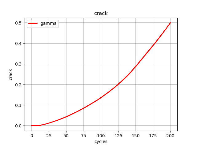
Plot: Cycles vs. Normalized Crack Length#
This plot visualizes the relationship between the number of cycles and the normalized crack length during the simulation. The crack length is represented by $gamma(phi) = int_{Omega} frac{1}{2l} phi^2 + frac{l}{2} |nabla phi|^2 d Omega$, and the plot normalizes this variable by dividing it by the maximum value of gamma to scale the crack length between 0 and 0.5.
The red curve represents the evolution of the crack length as a function of the number of cycles, showing how the crack propagates with each loading cycle.
cycles: The x-axis represents the number of loading cycles.
The y-axis represents the normalized crack length, where the maximum value of gamma is scaled to 0.5 to represent the crack growth.
This plot is useful for examining the crack growth behavior over multiple cycles.
fig, ax_r = plt.subplots()

ax_r.plot(cycles, S.energy_files["total.energy"]["gamma"] / max(S.energy_files["total.energy"]["gamma"]) * 0.5, 'r-', linewidth=2.0, label='gamma')

ax_r.grid(color='k', linestyle='-', linewidth=0.3)
ax_r.set_xlabel('cycles')
ax_r.set_ylabel('crack')
ax_r.set_title('crack')
ax_r.legend()

plt.show()
Total running time of the script: (0 minutes 0.846 seconds)