Three point bending test

A well-known benchmark simulation in fracture mechanics is performed, relying on the simulation conducted by [Miehe]. This simulation considers an anisotropic formulation with spectral energy decomposition.

A rectangular plate with an initial notch positioned at the bottom center is shown in the figure below. This beam is supported at its ends, as shown in the figure. The bottom left part is fixed in all directions, while the bottom right part is fixed in the vertical direction. A vertical displacement is applied at the top. The geometry and boundary conditions are depicted in the figure. We discretize the model with triangular elements, refining the areas (element size h) where crack evolution is expected. The element size h must be sufficiently small to avoid mesh dependencies.

#                            u||||
#                             \/\/
#            ------------------------------------*
#            |                                   |
#            |                                   |
#            |                                   |
#            |                 /\                |
#            *-----------------  ----------------*
#            /_\/_\        (0,0,0)          /_\/_\
#    |Y     ///////                         oo  oo
#    |
#    ---X
# Z /

The Young’s modulus, Poisson’s ratio, and the critical energy release rate are given in the table Properties. Young’s modulus \(E\) and Poisson’s ratio \(\nu\) can be represented with the Lamé parameters as: \(\lambda=\frac{E\nu}{(1+\nu)(1-2\nu)}\); \(\mu=\frac{E}{2(1+\nu)}\).

	VALUE	UNITS
E	20.8	kN/mm2
nu	0.3	[-]
Gc	0.0005	kN/mm
l	0.006	mm

[Miehe]

A phase field model for rate-independent crack propagation: Robust algorithmic implementation based on operator splits, https://doi.org/10.1016/j.cma.2010.04.011.

Import necessary libraries

import numpy as np
import matplotlib.pyplot as plt
import pyvista as pv
import dolfinx
import mpi4py
import petsc4py
import os

Import from phasefieldx package

from phasefieldx.Element.Phase_Field_Fracture.Input import Input
from phasefieldx.Element.Phase_Field_Fracture.solver.solver import solve
from phasefieldx.Boundary.boundary_conditions import bc_xy, bc_y, get_ds_bound_from_marker
from phasefieldx.PostProcessing.ReferenceResult import AllResults

Parameters Definition

Data is an input object containing essential parameters for simulation setup and result storage:

• E: Young’s modulus, set to 20.8 \(kN/mm^2\).

• nu: Poisson’s ratio, set to 0.3.

• Gc: Critical energy release rate, set to 0.0005 \(kN/mm\).

• l: Length scale parameter, set to 0.06 \(mm\).

• degradation: Specifies the degradation type. Options are “isotropic” or “anisotropic”.

• split_energy: Controls how the energy is split; options include “no” (default), “spectral,” or “deviatoric.” In this case an anisotropic model with spectral decomposition is considered.

• degradation_function: Specifies the degradation function; here, it is “quadratic.”

• irreversibility: Determines the irreversibility criterion; in this case, set to “miehe.”

• fatigue: Enables fatigue simulation when set to True.

• fatigue_degradation_function: Defines the function for fatigue degradation, set to “asymptotic.”

• fatigue_val: Fatigue parameter value (used only in fatigue simulations, not in this one).

• k: Stiffness penalty parameter, set to 0.0.

• min_stagger_iter: Minimum number of staggered iterations, set to 2.

• max_stagger_iter: Maximum number of staggered iterations, set to 500.

• stagger_error_tol: Error tolerance for staggered iterations, set to 1e-8.

• save_solution_xdmf and save_solution_vtu: Specify the file formats to save displacement results. In this case, results are saved as .vtu files.

• results_folder_name: Name of the folder for saving results. If it exists, it will be replaced with a new empty folder.

Data = Input(E=20.8,     # young modulus
             nu=0.3,     # poisson
             Gc=0.0005,  # critical energy release rate
             l=0.06,     # lenght scale parameter
             degradation="anisotropic",  # "isotropic" "anisotropic"
             split_energy="spectral",   # "spectral" "deviatoric"
             degradation_function="quadratic",
             irreversibility="miehe",  # "miehe"
             fatigue=False,
             fatigue_degradation_function="asymptotic",
             fatigue_val=0.05625,
             k=0.0,
             save_solution_xdmf=False,
             save_solution_vtu=True,
             results_folder_name="1714_Three_point_bending")

Mesh Definition

The mesh is generated using Gmsh and saved as a ‘mesh.msh’ file. For more details on how to create the mesh, refer to the Examples gmsh “.geo” files examples. The following lines

msh_file = os.path.join("mesh", "three_point_bending_test.msh") # Path to the mesh file
gdim = 2                                     # Geometric dimension of the mesh
gmsh_model_rank = 0                          # Rank of the Gmsh model in a parallel setting
mesh_comm = mpi4py.MPI.COMM_WORLD            # MPI communicator for parallel computation

The mesh, cell markers, and facet markers are extracted from the ‘mesh.msh’ file using the read_from_msh function.

mesh_data = dolfinx.io.gmsh.read_from_msh(msh_file, mesh_comm, gmsh_model_rank, gdim)
msh = mesh_data.mesh
cell_markers = mesh_data.cell_tags
facet_markers = mesh_data.facet_tags

fdim = msh.topology.dim - 1 # Dimension of the mesh facets

Boundary Identification Functions

These functions identify points on the specific boundaries of the domain where boundary conditions will be applied. The bottom_left function checks if a point lies on the bottom left boundary, returning True for points where y=0 and x is less than -3.9, and False otherwise. Similarly, the bottom_right function identifies points on the bottom right boundary, returning True for points where y=0 and x is greater than 3.9, and False otherwise. The top function identifies points on the top boundary, returning True for points where y=2, and x is between -0.25 and 0.25, and False otherwise.

This approach ensures that boundary conditions are applied to specific parts of the mesh, which helps in defining the simulation’s physical constraints.

def bottom_left(x):
    return np.logical_and(np.isclose(x[1], 0), np.less(x[0], -3.9))

def bottom_right(x):
    return np.logical_and(np.isclose(x[1], 0), np.greater(x[0], 3.9))

def top(x):
    return np.logical_and(np.logical_and(np.isclose(x[1], 2), np.greater(x[0], -0.25)), np.less(x[0], 0.25))

Using the bottom and top functions, we locate the facets on the bottom and top sides of the mesh, where \(y = 0\) and \(y = 1\), respectively. The locate_entities_boundary function returns an array of facet indices representing these identified boundary entities.

bottom_left_facet_marker = dolfinx.mesh.locate_entities_boundary(msh, fdim, bottom_left)
bottom_right_facet_marker = dolfinx.mesh.locate_entities_boundary(msh, fdim, bottom_right)
top_facet_marker = dolfinx.mesh.locate_entities_boundary(msh, fdim, top)

The get_ds_bound_from_marker function generates a measure for applying boundary conditions specifically to the facets identified by top_facet_marker and bottom_facet_marker, respectively. This measure is then assigned to ds_bottom and ds_top.

ds_bottom_left = get_ds_bound_from_marker(bottom_left_facet_marker, msh, fdim)
ds_bottom_right = get_ds_bound_from_marker(bottom_right_facet_marker, msh, fdim)
ds_top = get_ds_bound_from_marker(top_facet_marker, msh, fdim)

ds_list is an array that stores boundary condition measures along with names for each boundary, simplifying result-saving processes. Each entry in ds_list is formatted as [ds_, “name”], where ds_ represents the boundary condition measure, and “name” is a label used for saving. Here, ds_bottom and ds_top are labeled as “bottom” and “top”, respectively, to ensure clarity when saving results.

ds_list = np.array([
                   [ds_top, "top"],
                   [ds_bottom_left, "bottom_left"],
                   [ds_bottom_right, "bottom_right"],
                   ])

Function Space Definition

Define function spaces for displacement and phase-field using Lagrange elements.

V_u = dolfinx.fem.functionspace(msh, ("Lagrange", 1, (msh.geometry.dim, )))
V_phi = dolfinx.fem.functionspace(msh, ("Lagrange", 1))

Boundary Conditions

Dirichlet boundary conditions are defined as follows:

• bc_bottom_left: Constrains both x and y displacements on the bottom left boundary, ensuring that the leftmost bottom edge remains fixed.

• bc_bottom_right: Constrains only the vertical displacement (y-displacement) on the bottom right boundary, while allowing horizontal movement.

• bc_top: Constrains the vertical displacement (y-displacement) on the top boundary, while allowing horizontal movement.

These boundary conditions ensure that the relevant portions of the mesh are correctly fixed or allowed to move according to the simulation requirements.

bc_bottom_left = bc_xy(bottom_left_facet_marker, V_u, fdim)
bc_bottom_right = bc_y(bottom_right_facet_marker, V_u, fdim)
bc_top = bc_y(top_facet_marker, V_u, fdim)

The bcs_list_u variable is a list that stores all boundary conditions for the displacement field \(\boldsymbol u\). This list facilitates easy management of multiple boundary conditions and can be expanded if additional conditions are needed.

bcs_list_u = [bc_top, bc_bottom_left, bc_bottom_right]
bcs_list_u_names = ["top", "bottom_left", "bottom_right"]

Function: update_boundary_conditions

The update_boundary_conditions function dynamically updates the displacement boundary conditions at each time step. This allows for quasi-static analysis by incrementally adjusting the displacements applied to specific degrees of freedom.

Parameters:

• bcs: A list of boundary conditions, where each element corresponds to a boundary condition applied to a specific facet of the mesh.

• time: A scalar representing the current time step in the analysis.

Function Details:

• The displacement value val is computed based on the current time:

• For time <= 36, val increases linearly as val = dt0 * time, where dt0 is a small time step factor (10^-3), simulating gradual displacement along the y-axis.

• For time > 36, val increases more gradually as val = 36 * dt0 + (dt0 / 10) * (time - 36), which represents a slower displacement rate after the initial phase.

• This calculated value is assigned to the y-component of the displacement field on the top boundary by modifying bcs[0].g.value[1], where bcs[0] represents the top boundary condition. The displacement is negated to represent a displacement in the opposite direction.

Return Value:

• A tuple (0, val, 0) is returned, representing the incremental displacement vector:

• The first element (0) corresponds to no update for the x-displacement.

• The second element (val) is the calculated y-displacement.

• The third element (0) corresponds to no update for the z-displacement, applicable in 2D simulations.

Purpose:

• This function facilitates quasi-static analysis by applying controlled, time-dependent boundary displacements. It is essential for simulations that involve gradual loading or unloading, with a slower displacement evolution after the initial phase.

def update_boundary_conditions(bcs, time):
    dt0 = 10**-3
    if time <= 36:
        val = dt0 * time
    else:
        val = 36 * dt0 + dt0 / 10 * (time - 36)
    bcs[0].g.value[...] = petsc4py.PETSc.ScalarType(-val)
    return 0, val, 0


T_list_u = None
update_loading = None
f = None
T = dolfinx.fem.Constant(msh, petsc4py.PETSc.ScalarType((0.0, 0.0)))

Boundary Conditions for phase field

bcs_list_phi = []

Solver Call for a Phase-Field Fracture Problem

This section sets up and calls the solver for a phase-field fracture problem.

Key Points:

• The simulation is run for a final time of 150, with a time step of 1.0.

• The solver will manage the mesh, boundary conditions, and update the solution over the specified time steps.

Parameters:

• dt: The time step for the simulation, set to 1.0.

• final_time: The total simulation time, set to 200.0, which determines how long the problem will be solved.

• path: Optional parameter for specifying the folder where results will be saved; here it is set to None, meaning results will be saved to the default location.

Function Call:

The solve function is invoked with the following arguments:

• Data: Contains the simulation parameters and configurations.

• msh: The mesh representing the domain for the problem.

• final_time: The total duration of the simulation (200.0).

• V_u: Function space for the displacement field, \(\boldsymbol{u}\).

• V_phi: Function space for the phase field, \(\phi\).

• bcs_list_u: List of Dirichlet boundary conditions for the displacement field.

• bcs_list_phi: List of boundary conditions for the phase field (empty in this case).

• update_boundary_conditions: Function to update boundary conditions for the displacement field.

• f: The body force applied to the domain (if any).

• T_list_u: Time-dependent loading parameters for the displacement field.

• update_loading: Function to update loading parameters for the quasi-static analysis.

• ds_list: Boundary measures for integration over the domain boundaries.

• dt: The time step for the simulation.

• path: Directory for saving results (if specified).

This setup provides a framework for solving static problems with specified boundary conditions and loading parameters.

final_time = 150
dt = 1

Uncomment the following lines to run the solver with the specified parameters.

# solve(Data,
#       msh,
#       final_time,
#       V_u,
#       V_phi,
#       bcs_list_u,
#       bcs_list_phi,
#       update_boundary_conditions,
#       f,
#       T_list_u,
#       update_loading,
#       ds_list,
#       dt,
#       path=None,
#       bcs_list_u_names=bcs_list_u_names,
#       min_stagger_iter=2,
#       max_stagger_iter=1000,
#       stagger_error_tol=1e-6)

Load results

Once the simulation finishes, the results are loaded from the results folder. The AllResults class takes the folder path as an argument and stores all the results, including logs, energy, convergence, and DOF files. Note that it is possible to load results from other results folders to compare results. It is also possible to define a custom label and color to automate plot labels.

S = AllResults(Data.results_folder_name)
S.set_label('Simulation')
S.set_color('b')

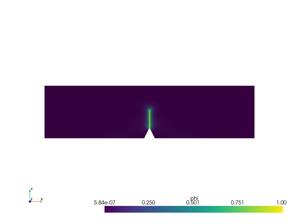
Plot: phase-field \(\phi\)

The phase-field result saved in the .vtu file is shown. For this, the file is loaded using PyVista.

file_vtu = pv.read(os.path.join(Data.results_folder_name, "paraview-solutions_vtu", "phasefieldx_p0_000065.vtu"))
file_vtu.plot(scalars='phi', cpos='xy', show_scalar_bar=True, show_edges=False)

Static Scene

Interactive Scene

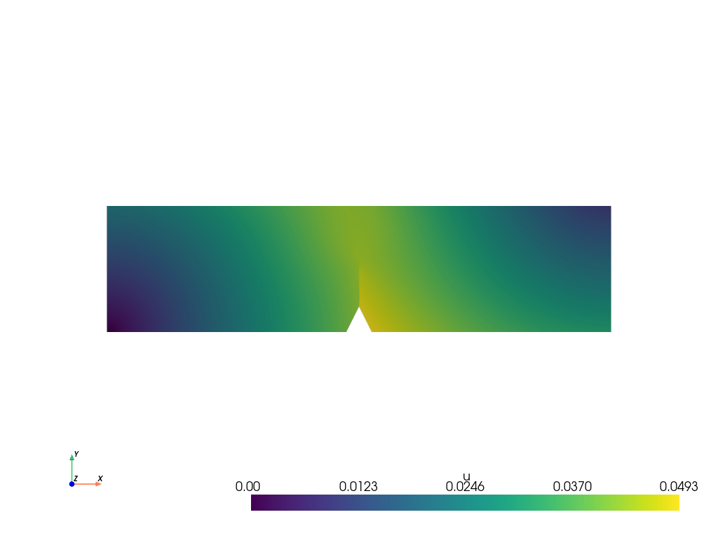
Plot: displacement \(\boldsymbol u\)

The displacements results saved in the .vtu file are shown. For this, the file is loaded using PyVista.

file_vtu.plot(scalars='u', cpos='xy', show_scalar_bar=True, show_edges=False)

plt.show()

Static Scene

Interactive Scene

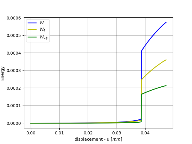
Plot: Displacement vs Fracture Energy

The vertical displacement is saved in S.dof_files[“top.dof”][“Uy”].

displacement = S.dof_files["top.dof"]["Uy"]

fig, energyW = plt.subplots()

energyW.plot(displacement, S.energy_files['total.energy']["W"], 'b-', linewidth=2.0, label=r'$W$')
energyW.plot(displacement, S.energy_files['total.energy']["W_phi"], 'y-', linewidth=2.0, label=r'$W_{\phi}$')
energyW.plot(displacement, S.energy_files['total.energy']["W_gradphi"], 'g-', linewidth=2.0, label=r'$W_{\nabla \phi}$')

energyW.grid(color='k', linestyle='-', linewidth=0.3)
energyW.set_xlabel('displacement - u $[mm]$')
energyW.set_ylabel('Energy')
energyW.legend()

<matplotlib.legend.Legend object at 0x73426e679000>

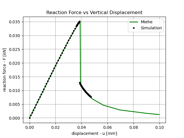
Plot: Force vs Vertical Displacement

Miehe = np.loadtxt(os.path.join("reference_solutions", "miehe_three_point.csv"))

fig, ax_reaction = plt.subplots()

ax_reaction.plot(Miehe[:, 0], Miehe[:, 1], 'g-', linewidth=2.0, label='Miehe')
ax_reaction.plot(displacement, -S.reaction_files['top.reaction']["Ry"], 'k.', linewidth=2.0, label=S.label)
ax_reaction.grid(color='k', linestyle='-', linewidth=0.3)
ax_reaction.set_xlabel('displacement - u $[mm]$')
ax_reaction.set_ylabel('reaction force - F $[kN]$')
ax_reaction.set_title('Reaction Force vs Vertical Displacement')
ax_reaction.legend()

<matplotlib.legend.Legend object at 0x73426e6d38e0>

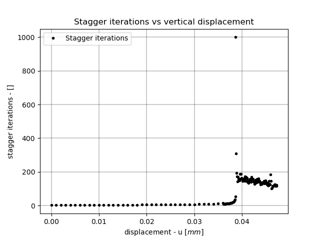
Plot: Staggered Iterations vs Vertical Displacement

fig, ax_convergence = plt.subplots()

ax_convergence.plot(displacement, S.convergence_files["phasefieldx.conv"]["stagger"], 'k.', linewidth=2.0, label='Stagger iterations')

ax_convergence.grid(color='k', linestyle='-', linewidth=0.3)
ax_convergence.set_xlabel('displacement - u $[mm]$')
ax_convergence.set_ylabel('stagger iterations - []')
ax_convergence.set_title('Stagger iterations vs vertical displacement')
ax_convergence.legend()

plt.show()