One Element tension anisotropic (spectral)

In this example, we consider a phase-field fracture simulation. The theoretical basis for this model is outlined in detail in (Phase-field fracture). Unlike the previous case (One Element tension Isotropic), this simulation includes split energy, which the use of the anisotropic model with spectral decomposition. The setup involves a simple model comprising a single four-node element with dimensions of 1x1 mm. The bottom nodes are fully constrained in both directions, while the top nodes are allowed to slide vertically.

#          u /\        /\
#            ||        ||
#     (0, 1) *----------* (1, 1)
#            |          |
#            |          |
#            |          |
#            |          |
#            |          |
#     (0, 0) *----------* (0, 1)
#            /_\       /_\
#     |Y    ////       ///
#     |
#     *---X

The Young’s modulus, Poisson’s ratio, and the critical energy release rate are given in the table Properties. Young’s modulus \(E\) and Poisson’s ratio \(\nu\) can be represented with the Lamé parameters as: \(\lambda=\frac{E\nu}{(1+\nu)(1-2\nu)}\); \(\mu=\frac{E}{2(1+\nu)}\).

Properties

	VALUE	UNITS
E	210	kN/mm2
nu	0.3	[-]
Gc	0.005	kN/mm
l	0.1	mm

In this case, due to the discretization, it is possible to obtain an analytical solution for the isotropic model by solving \(\phi\) from the given equations. The term \(|\nabla \phi|^2\) vanishes due to the discretization as explained by Molnar [MOLNAR201727] and Miehe [Miehe1] in the appendix.

\[\phi = \frac{2 \psi_a}{\frac{G_c}{l}+2\psi_a}=\frac{2 H}{\frac{G_c}{l}+2H}\]

\[\begin{split}\\sigma_y = \\sigma_{a}(1-\\phi)^2 + \\sigma_{b}\end{split}\]

[MOLNAR201727]

2D and 3D Abaqus implementation of a robust staggered phase-field solution for modeling brittle fracture, https://doi.org/10.1016/j.finel.2017.03.002

[Miehe1]

A phase field model for rate-independent crack propagation: Robust algorithmic implementation based on operator splits, https://doi.org/10.1016/j.cma.2010.04.011.

Import necessary libraries

import numpy as np
import matplotlib.pyplot as plt
import pyvista as pv
import dolfinx
import mpi4py
import petsc4py
import os

Import from phasefieldx package

from phasefieldx.Element.Phase_Field_Fracture.Input import Input
from phasefieldx.Element.Phase_Field_Fracture.solver.solver import solve
from phasefieldx.Boundary.boundary_conditions import bc_xy, bc_y, get_ds_bound_from_marker
from phasefieldx.PostProcessing.ReferenceResult import AllResults

Parameters Definition

Data is an input object containing essential parameters for simulation setup and result storage:

• E: Young’s modulus, set to 210 \(kN/mm^2\).

• nu: Poisson’s ratio, set to 0.3.

• Gc: Critical energy release rate, set to 0.005 \(kN/mm\).

• l: Length scale parameter, set to 0.1 \(mm\).

• degradation: Specifies the degradation type. Options are “isotropic” or “anisotropic”.

• split_energy: Controls how the energy is split; options include “no” (default), “spectral,” or “deviatoric.”

• degradation_function: Specifies the degradation function; here, it is “quadratic.”

• irreversibility: Determines the irreversibility criterion; in this case, set to “miehe.” We consider anisotropic (spectral) degradation and irreversibility as proposed by Miehe.

• fatigue: Enables fatigue simulation when set to True.

• fatigue_degradation_function: Defines the function for fatigue degradation, set to “asymptotic.”

• fatigue_val: Fatigue parameter value (used only in fatigue simulations, not in this one).

• k: Stiffness penalty parameter, set to 0.0.

• min_stagger_iter: Minimum number of staggered iterations, set to 2.

• max_stagger_iter: Maximum number of staggered iterations, set to 500.

• stagger_error_tol: Error tolerance for staggered iterations, set to 1e-8.

• save_solution_xdmf and save_solution_vtu: Specify the file formats to save displacement results. In this case, results are saved as .vtu files.

• results_folder_name: Name of the folder for saving results. If it exists, it will be replaced with a new empty folder.

Data = Input(E=210.0,   # young modulus
             nu=0.3,    # poisson
             Gc=0.005,  # critical energy release rate
             l=0.1,     # lenght scale parameter
             degradation="anisotropic",  # "isotropic" "anisotropic"
             split_energy="spectral",       # "spectral" "deviatoric"
             degradation_function="quadratic",
             irreversibility="miehe",  # "miehe"
             fatigue=False,
             fatigue_degradation_function="asymptotic",
             fatigue_val=0.0,
             k=0.0,
             save_solution_xdmf=False,
             save_solution_vtu=True,
             results_folder_name="1702_One_element_anisotropic_spectral")

Mesh Definition

Create a 1x1 mm rectangular mesh with one quadrilateral element

msh = dolfinx.mesh.create_rectangle(
    mpi4py.MPI.COMM_WORLD,                     # MPI communicator
    [np.array([0, 0]), np.array([1, 1])],     # Domain corners: bottom-left and top-right
    [1, 1],                                   # Number of elements in x and y directions
    cell_type=dolfinx.mesh.CellType.quadrilateral  # Specify quadrilateral cell type
)

Boundary Identification Functions

These functions identify points on the bottom and top sides of the domain where boundary conditions will be applied. The bottom function checks if a point lies on the bottom boundary by returning True for points where y=0 and False otherwise. Similarly, the top function identifies points on the top boundary by returning True for points where y=1 and False otherwise.

This approach ensures boundary conditions are applied only to the relevant parts of the mesh.

def bottom(x):
    return np.isclose(x[1], 0)

def top(x):
    return np.isclose(x[1], 1)


fdim = msh.topology.dim - 1 # Dimension of the mesh facets

Using the bottom and top functions, we locate the facets on the bottom and top sides of the mesh, where \(y = 0\) and \(y = 1\), respectively. The locate_entities_boundary function returns an array of facet indices representing these identified boundary entities.

bottom_facet_marker = dolfinx.mesh.locate_entities_boundary(msh, fdim, bottom)
top_facet_marker = dolfinx.mesh.locate_entities_boundary(msh, fdim, top)

The get_ds_bound_from_marker function generates a measure for applying boundary conditions specifically to the facets identified by top_facet_marker and bottom_facet_marker, respectively. This measure is then assigned to ds_bottom and ds_top.

ds_bottom = get_ds_bound_from_marker(top_facet_marker, msh, fdim)
ds_top = get_ds_bound_from_marker(top_facet_marker, msh, fdim)

ds_list is an array that stores boundary condition measures along with names for each boundary, simplifying result-saving processes. Each entry in ds_list is formatted as [ds_, “name”], where ds_ represents the boundary condition measure, and “name” is a label used for saving. Here, ds_bottom and ds_top are labeled as “bottom” and “top”, respectively, to ensure clarity when saving results.

ds_list = np.array([
                   [ds_top, "top"],
                   [ds_bottom, "bottom"],
                   ])

Function Space Definition

Define function spaces for displacement and phase-field using Lagrange elements.

V_u = dolfinx.fem.functionspace(msh, ("Lagrange", 1, (msh.geometry.dim, )))
V_phi = dolfinx.fem.functionspace(msh, ("Lagrange", 1))

Boundary Conditions

Dirichlet boundary conditions are defined as follows:

• bc_bottom: Constrains both x and y displacements to 0 on the bottom boundary,

ensuring that the bottom edge remains fixed. - bc_top: Constrains the x displacement, while the vertical displacement on the top boundary is updated dynamically in the quasi-static solver to impose the desired vertical displacement.

bc_bottom = bc_xy(bottom_facet_marker, V_u, fdim)
bc_top = bc_xy(top_facet_marker, V_u, fdim)

The bcs_list_u variable is a list that stores all boundary conditions for the displacement field \(\boldsymbol u\). This list facilitates easy management of multiple boundary conditions and can be expanded if additional conditions are needed.

bcs_list_u = [bc_top, bc_bottom]
bcs_list_u_names = ["top", "bottom"]

Function: update_boundary_conditions

The update_boundary_conditions function updates the displacement boundary conditions dynamically at each time step, enabling quasi-static analysis by incrementally adjusting the displacements applied to specific degrees of freedom.

Parameters:

• bcs: A list of boundary conditions, where each element corresponds to a boundary condition applied to a specific facet of the mesh.

• time: A scalar representing the current time step in the analysis.

Function Details:

• The displacement value val is computed based on the current time:

• For time <= 50, val increases linearly as val = 0.0003 * time, simulating gradual displacement along the y-axis.

• For 50 < time <= 150, val decreases linearly as val = -0.0003 * (time - 50) + 0.015.

• For time > 150, val resumes a positive linear increase with a slight offset, calculated as val = 0.0003 * (time - 150) - 0.015.

• This calculated value is assigned to the y-component of the displacement field on the top boundary by modifying bcs[0].g.value[1], where bcs[0] represents the top boundary condition.

Return Value:

• A tuple (0, val, 0) is returned, representing the incremental displacement vector:

• The first element (0) corresponds to no update for the x-displacement.

• The second element (val) is the calculated y-displacement.

• The third element (0) corresponds to no update for the z-displacement, applicable in 2D simulations.

Purpose:

• This function facilitates quasi-static analysis by applying controlled, time-dependent boundary displacements. It is essential for simulations that involve gradual loading or unloading, with periodic displacement adjustments.

def update_boundary_conditions(bcs, time):
    if time <= 50:
        val = 0.0003 * time
    elif time <= 150:
        val = -0.0003 * (time - 50) + 0.015
    else:
        val = 0.0003 * (time - 150) - 0.015

    bcs[0].g.value[1] = petsc4py.PETSc.ScalarType(val)
    return 0, val, 0


bcs_list_phi = []
T_list_u = None
update_loading = None
f = None

Solver Call for a Phase-Field Fracture Problem

This section sets up and calls the solver for a phase-field fracture problem.

Key Points:

• The simulation is run for a final time of 200, with a time step of 1.0.

• The solver will manage the mesh, boundary conditions, and update the solution over the specified time steps.

Parameters:

• dt: The time step for the simulation, set to 1.0.

• final_time: The total simulation time, set to 200.0, which determines how long the problem will be solved.

• path: Optional parameter for specifying the folder where results will be saved; here it is set to None, meaning results will be saved to the default location.

Function Call: The solve function is invoked with the following arguments:

• Data: Contains the simulation parameters and configurations.

• msh: The mesh representing the domain for the problem.

• final_time: The total duration of the simulation (200.0).

• V_u: Function space for the displacement field, \(\boldsymbol{u}\).

• V_phi: Function space for the phase field, \(\phi\).

• bcs_list_u: List of Dirichlet boundary conditions for the displacement field.

• bcs_list_phi: List of boundary conditions for the phase field (empty in this case).

• update_boundary_conditions: Function to update boundary conditions for the displacement field.

• f: The body force applied to the domain (if any).

• T_list_u: Time-dependent loading parameters for the displacement field.

• update_loading: Function to update loading parameters for the quasi-static analysis.

• ds_list: Boundary measures for integration over the domain boundaries.

• dt: The time step for the simulation.

• path: Directory for saving results (if specified).

This setup provides a framework for solving static problems with specified boundary conditions and loading parameters.

dt = 1.0
final_time = 200.0

solve(Data,
      msh,
      final_time,
      V_u,
      V_phi,
      bcs_list_u,
      bcs_list_phi,
      update_boundary_conditions,
      f,
      T_list_u,
      update_loading,
      ds_list,
      dt,
      path=None,
      bcs_list_u_names=bcs_list_u_names,
      min_stagger_iter=2,
      max_stagger_iter=500,
      stagger_error_tol=1e-8,)

All specified files deleted successfully.
All specified folders and their contents deleted successfully.
All specified folders and their contents deleted successfully.

Load results

Once the simulation finishes, the results are loaded from the results folder. The AllResults class takes the folder path as an argument and stores all the results, including logs, energy, convergence, and DOF files. Note that it is possible to load results from other results folders to compare results. It is also possible to define a custom label and color to automate plot labels.

S = AllResults(Data.results_folder_name)
S.set_label('Simulation')
S.set_color('b')

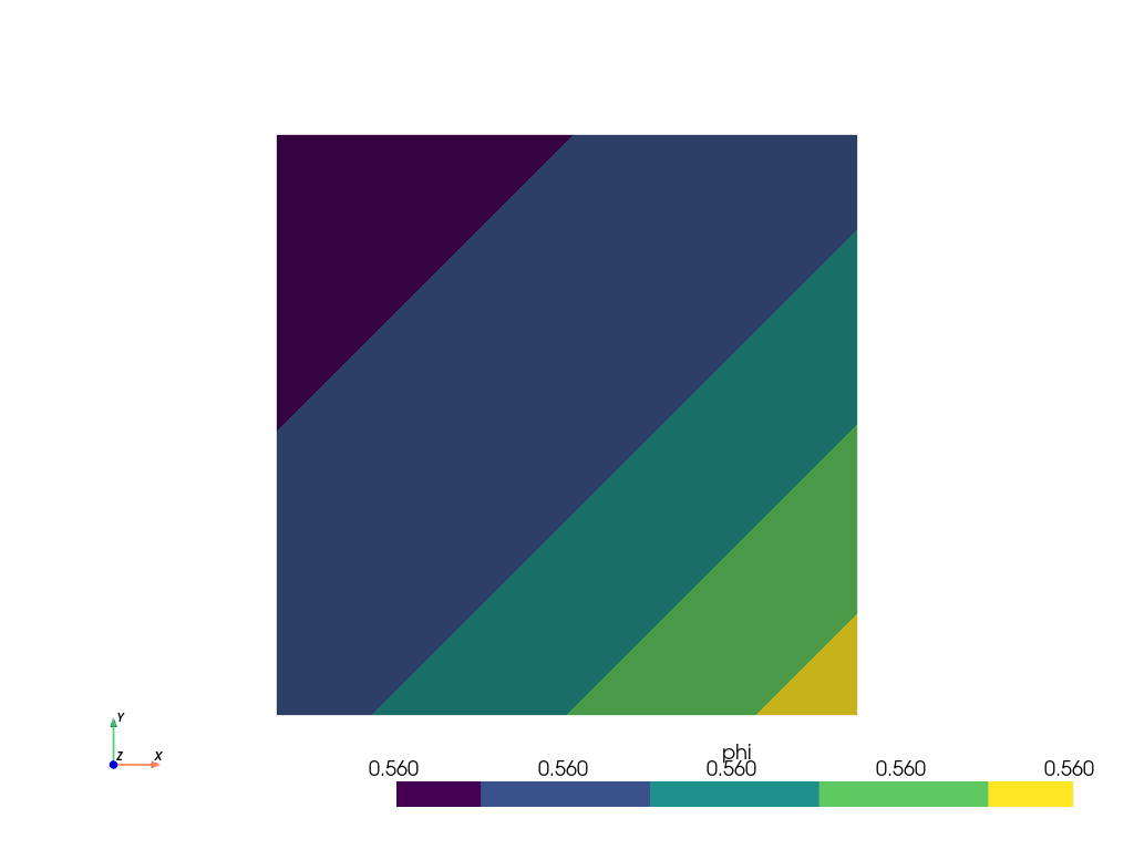
Plot: phase-field \(\phi\)

The phase-field result saved in the .vtu file is shown. For this, the file is loaded using PyVista.

file_vtu = pv.read(os.path.join(Data.results_folder_name, "paraview-solutions_vtu", "phasefieldx_p0_000080.vtu"))
file_vtu.plot(scalars='phi', cpos='xy', show_scalar_bar=True, show_edges=False)

Static Scene

Interactive Scene

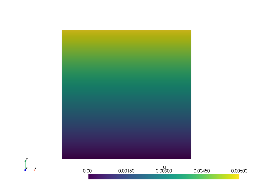
Plot: displacement \(\boldsymbol u\)

The displacements results saved in the .vtu file are shown. For this, the file is loaded using PyVista.

file_vtu = pv.read(os.path.join(Data.results_folder_name, "paraview-solutions_vtu", "phasefieldx_p0_000080.vtu"))
file_vtu.plot(scalars='u', cpos='xy', show_scalar_bar=True, show_edges=False)

Static Scene

Interactive Scene

Vertical Displacement

Compute and plot the vertical displacement.

displacement = S.dof_files["top.dof"]["Uy"]

Plot time vs reaction force

fig, ax = plt.subplots()

ax.plot(displacement, S.color + '.', linewidth=2.0, label=S.label)

ax.grid(color='k', linestyle='-', linewidth=0.3)
ax.set_xlabel('time')
ax.set_ylabel('displacement - u $[mm]$')

ax.legend()

<matplotlib.legend.Legend object at 0x73426e599120>

Vertical displacement vs. Reaction Force

Plot the vertical displacement versus the reaction force.

fig, ax = plt.subplots()

ax.plot(displacement, S.reaction_files['top.reaction']["Ry"], S.color + '.', linewidth=2.0, label=S.label)

ax.grid(color='k', linestyle='-', linewidth=0.3)
ax.set_xlabel('displacement - u $[mm]$')
ax.set_ylabel('reaction force - F $[kN]$')
ax.legend()

<matplotlib.legend.Legend object at 0x73426e79f640>

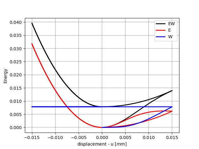
Plot Displacement vs. Energy

Plot the displacement versus the total energy.

fig, energy = plt.subplots()

energy.plot(displacement, S.energy_files['total.energy']["EplusW"], 'k-', linewidth=2.0, label='EW')
energy.plot(displacement, S.energy_files['total.energy']["E"], 'r-', linewidth=2.0, label='E')
energy.plot(displacement, S.energy_files['total.energy']["W"], 'b-', linewidth=2.0, label='W')

energy.legend()
energy.grid(color='k', linestyle='-', linewidth=0.3)
energy.set_xlabel('displacement - u $[mm]$')
energy.set_ylabel('Energy')

Text(24.847222222222214, 0.5, 'Energy')

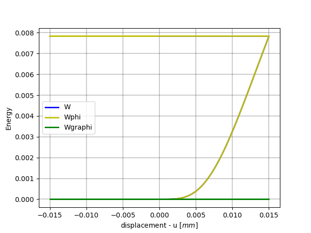
Plot Displacement vs. W Fracture Energy

Plot the displacement versus the fracture energy components.

fig, energyW = plt.subplots()

energyW.plot(displacement, S.energy_files['total.energy']["W"], 'b-', linewidth=2.0, label='W')
energyW.plot(displacement, S.energy_files['total.energy']["W_phi"], 'y-', linewidth=2.0, label='Wphi')
energyW.plot(displacement, S.energy_files['total.energy']["W_gradphi"], 'g-', linewidth=2.0, label='Wgraphi')

energyW.grid(color='k', linestyle='-', linewidth=0.3)
energyW.set_xlabel('displacement - u $[mm]$')
energyW.set_ylabel('Energy')
energyW.legend()

plt.show()