Note
Go to the end to download the full example code.
Representation of a Cracked Plate#
In this example, we solve a boundary value problem for a cracked plate using the phase-field model (Crack Surface Density Functional). The crack is represented by the phase field variable, following the approach presented by [Miehe]. We apply a boundary condition of \(\phi = 1\), representing the broken part of the material, and simulate the crack representation with different length scale values.
To exploit symmetry, only half of the plate is simulated, and we reflect the results to show the full solution. This allows us to reduce computational cost while capturing the entire domain’s behavior.
#
#        *---------------*  -
#        |               |  |
#        |               | 0.5
#        | phi=1         |  |
#        *........-------*  -
#        |<-0.5->|
#     |Y
#     |
#     *---X
A phase field model for rate-independent crack propagation: Robust algorithmic implementation based on operator splits, https://doi.org/10.1016/j.cma.2010.04.011.
Import necessary libraries#
import numpy as np
import matplotlib.pyplot as plt
import pyvista as pv
import dolfinx
import mpi4py
import os
Import from phasefieldx package#
from phasefieldx.Element.Phase_Field.Input import Input
from phasefieldx.Element.Phase_Field.solver.solver import solve
from phasefieldx.Boundary.boundary_conditions import bc_phi, get_ds_bound_from_marker
from phasefieldx.PostProcessing.ReferenceResult import AllResults
Parameter Definition#
In this section, we define various length scale parameters, denoted as \(l\), which will be used in the simulations. We will run three simulations with different values of \(l\)—specifically, \(l=1.0\), \(l=0.25\), and \(l=0.05\)—which will correspond to three distinct input classes. These length scale parameters control the smoothness of the crack surface: smaller values of \(l\) lead to sharper cracks, while larger values result in smoother cracks. The phase-field results will be saved in VTU format for subsequent visualization. For further details about the input class, please refer to Crack surface density functional.
Data1 = Input(l=1.0,
              save_solution_xdmf=False,
              save_solution_vtu=True,
              results_folder_name="2001_regularized_crack_surface_l1")

Data025 = Input(l=0.25,
                save_solution_xdmf=False,
                save_solution_vtu=True,
                results_folder_name="2001_regularized_crack_surface_l025")

Data005 = Input(l=0.05,
                save_solution_xdmf=False,
                save_solution_vtu=True,
                results_folder_name="2001_regularized_crack_surface_l005")
Mesh definition#
We define the mesh for the simulations. The mesh covers a rectangular domain with dimensions lx=1.0 and ly=0.5. The mesh is subdivided into divx and divy divisions along the x and y axes, respectively. In this case, 100 divisions are made in the x-direction, and 50 in the y-direction, giving us sufficient resolution for the crack representation.
divx, divy = 100, 50
lx, ly = 1.0, 0.5
Create a 2D mesh using the defined parameters.
msh = dolfinx.mesh.create_rectangle(mpi4py.MPI.COMM_WORLD,
                                    [np.array([0, 0]),
                                     np.array([lx, ly])],
                                    [divx, divy],
                                    cell_type=dolfinx.mesh.CellType.quadrilateral)
Bottom boundary Identification#
This function identifies points on the bottom side of the domain where the boundary condition will be applied. Specifically, it returns True for points where y=0 and x<0.5; and False otherwise. This allows us to selectively apply boundary conditions only to this part of the mesh.
def bottom(x):
    return np.logical_and(np.isclose(x[1], 0), np.less(x[0], 0.5))
fdim represents the dimension of the boundary facets on the mesh, which is one less than the mesh’s overall dimensionality (msh.topology.dim). For example, if the mesh is 2D, fdim will be 1, representing 1D boundary edges.
fdim = msh.topology.dim - 1
Using the bottom function, we locate the facets on the bottom boundary side of the mesh. The locate_entities_boundary function returns an array of facet indices that represent the identified boundary entities.
bottom_facet_marker = dolfinx.mesh.locate_entities_boundary(msh, fdim, bottom)
get_ds_bound_from_marker is a function that generates a measure for integrating boundary conditions specifically on the facets identified by bottom_facet_marker. This measure is assigned to ds_bottom and will be used for applying boundary conditions on the left side.
ds_bottom = get_ds_bound_from_marker(bottom_facet_marker, msh, fdim)
ds_list is an array that stores boundary condition measures and associated names for each boundary to facilitate result-saving processes. Each entry in ds_list is an array in the form [ds_, “name”], where ds_ is the boundary condition measure, and “name” is a label for saving purposes. Here, ds_bottom is labeled as “bottom” for clarity when saving results.
ds_list = np.array([
                   [ds_bottom, "bottom"],
                   ])
Function Space Definition#
Define function spaces for the phase-field using Lagrange elements of degree 1.
V_phi = dolfinx.fem.functionspace(msh, ("Lagrange", 1))
Boundary Condition Setup for Scalar Field \(\phi\)#
We define and apply a Dirichlet boundary condition for the scalar field \(\phi\) on the bottom boundary side of the mesh, setting \(\phi = 1\) on this boundary. This setup is for a simple, static linear problem, meaning the boundary conditions and loading are constant and do not change throughout the simulation.
bc_phi is a function that creates a Dirichlet boundary condition on a specified facet of the mesh for the scalar field \(\phi\).
bcs_list_phi is a list that stores all the boundary conditions for \(\phi\), facilitating easy management and extension of conditions if needed.
update_boundary_conditions and update_loading are set to None as they are unused in this static case with constant boundary conditions and loading.
bc_bottom = bc_phi(bottom_facet_marker, V_phi, fdim, value=1.0)
bcs_list_phi = [bc_bottom]
update_boundary_conditions = None
update_loading = None
Solver Call for a Static Linear Problem#
We define the parameters for a simple, static linear boundary value problem with a final time t = 1.0 and a time step Δt = 1.0. Although this setup includes time parameters, they are primarily used for structural consistency with a generic solver function and do not affect the result, as the problem is linear and time-independent.
Parameters:
final_time: The end time for the simulation, set to 1.0.
dt: The time step for the simulation, set to 1.0. In a static context, this
only provides uniformity with dynamic cases but does not change the results. - path: Optional path for saving results; set to None here to use the default. - quadrature_degree: Defines the accuracy of numerical integration; set to 2 for this problem.
Function Call: The solve function is called with:
Data: Simulation data and parameters.
msh: Mesh of the domain.
V_phi: Function space for phi.
bcs_list_phi: List of boundary conditions.
update_boundary_conditions, update_loading: Set to None as they are unused in this static problem.
ds_list: Boundary measures for integration on specified boundaries.
dt and final_time to define the static solution time window.
final_time = 1.0
dt = 1.0
Simulation for \(l=1\)
solve(Data1,
      msh,
      final_time,
      V_phi,
      bcs_list_phi,
      update_boundary_conditions,
      update_loading,
      ds_list,
      dt,
      path=None,
      quadrature_degree=2)

S1 = AllResults(Data1.results_folder_name)
S1.set_label('$l_1$')
All specified files deleted successfully.
All specified folders and their contents deleted successfully.
All specified folders and their contents deleted successfully.
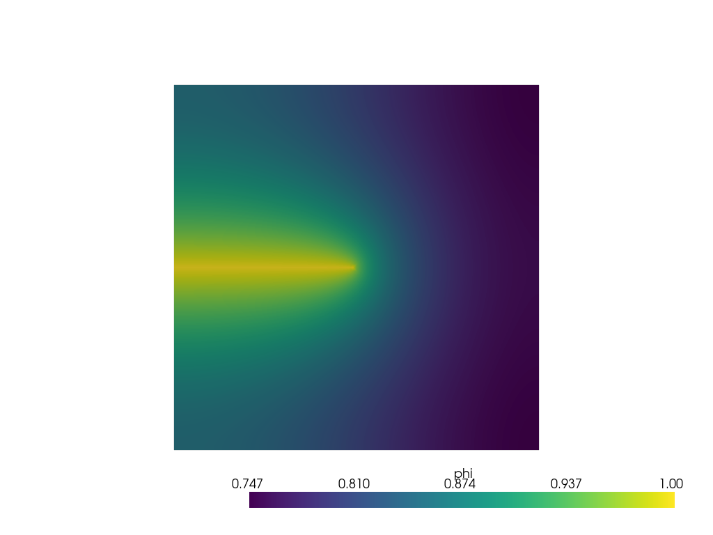
Plot phase-field \(\phi\) for \(l=1\)
file_vtu = pv.read(os.path.join(Data1.results_folder_name, "paraview-solutions_vtu", "phasefieldx_p0_000000.vtu"))
file_vtu_reflected = file_vtu.reflect((0, 1, 0), point=(0, 0, 0))
p = pv.Plotter()
p.add_mesh(file_vtu, show_edges=False)
p.add_mesh(file_vtu_reflected, show_edges=False)
p.camera_position = 'xy'
p.show()
Simulation for \(l=0.25\)
solve(Data025,
      msh,
      final_time,
      V_phi,
      bcs_list_phi,
      update_boundary_conditions,
      update_loading,
      ds_list,
      dt,
      path=None,
      quadrature_degree=2)

S025 = AllResults(Data025.results_folder_name)
S025.set_label('$l_025$')
All specified files deleted successfully.
All specified folders and their contents deleted successfully.
All specified folders and their contents deleted successfully.
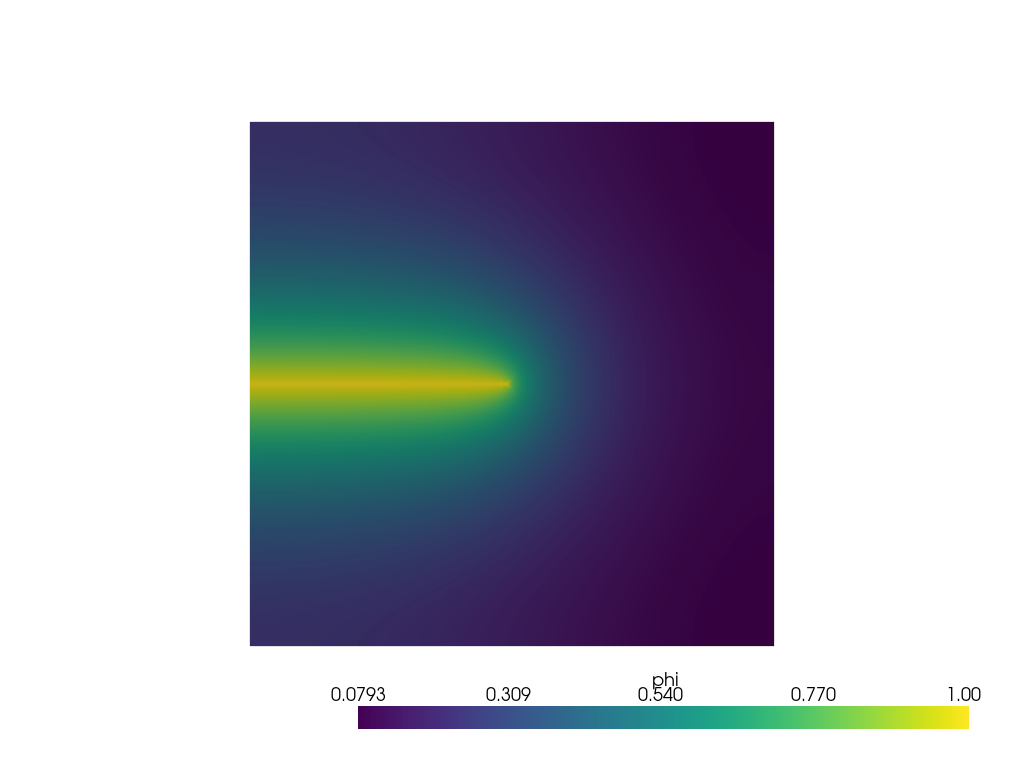
Plot phase-field \(\phi\) for \(l=0.25\)
file_vtu = pv.read(os.path.join(Data025.results_folder_name, "paraview-solutions_vtu", "phasefieldx_p0_000000.vtu"))
file_vtu_reflected = file_vtu.reflect((0, 1, 0), point=(0, 0, 0))

p = pv.Plotter()
p.add_mesh(file_vtu, show_edges=False)
p.add_mesh(file_vtu_reflected, show_edges=False)
p.camera_position = 'xy'
p.show()
Simulation for \(l=0.05\)
solve(Data005,
      msh,
      final_time,
      V_phi,
      bcs_list_phi,
      update_boundary_conditions,
      update_loading,
      ds_list,
      dt,
      path=None,
      quadrature_degree=2)
S005 = AllResults(Data005.results_folder_name)
S005.set_label('$l_005$')
All specified files deleted successfully.
All specified folders and their contents deleted successfully.
All specified folders and their contents deleted successfully.
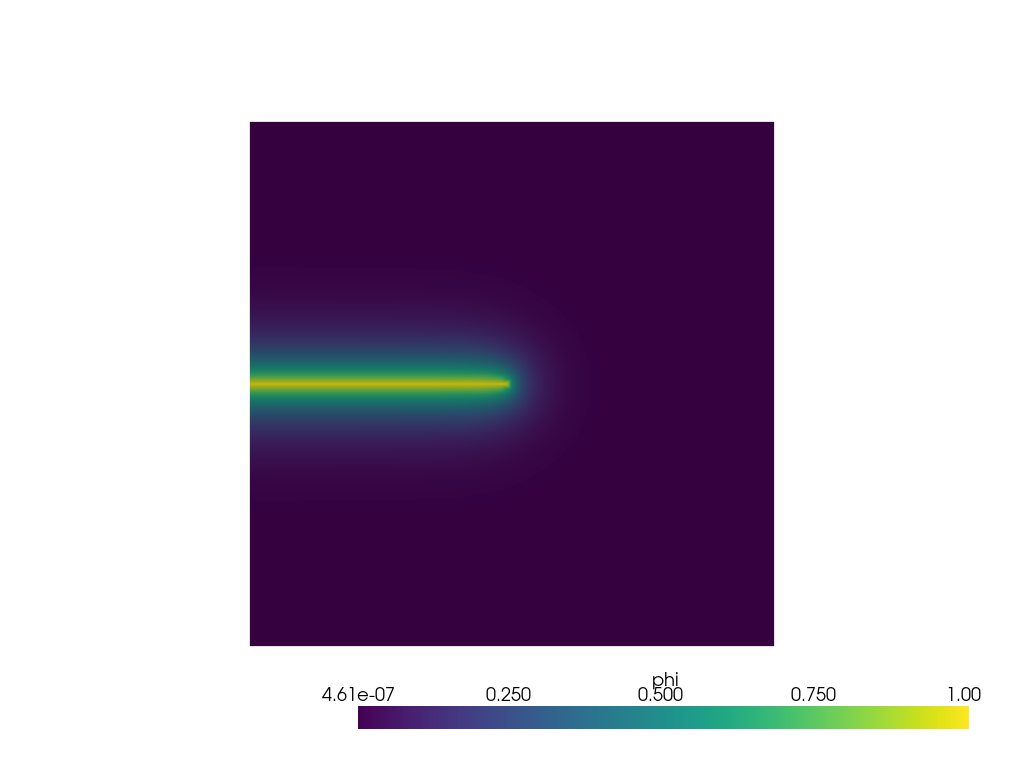
Plot phase-field \(\phi\) for \(l=0.05\)
file_vtu = pv.read(os.path.join(Data005.results_folder_name, "paraview-solutions_vtu", "phasefieldx_p0_000000.vtu"))
file_vtu_reflected = file_vtu.reflect((0, 1, 0), point=(0, 0, 0))

p = pv.Plotter()
p.add_mesh(file_vtu, show_edges=False)
p.add_mesh(file_vtu_reflected, show_edges=False)
p.camera_position = 'xy'
p.show()
Total running time of the script: (0 minutes 3.005 seconds)