Symmetry: Single edge notched tension test

A well-known benchmark simulation in fracture mechanics is performed, based on the simulation conducted by Miehe et al.[1]. This simulation employs an anisotropic formulation with spectral energy decomposition, though we have also repeated the simulations with an isotropic formulation.

The setup is identical to that presented in (Single edge notched tension test), but in this case, taking advantage of the specimen’s symmetric nature, only half of the domain is considered, as shown in the figure below.

#           u/\/\/\/\/\/\      u/\/\/\/\/\/\
#            ||||||||||||       ||||||||||||
#            *----------*       *----------*
#            |          |       |          |
#            | a=0.5    |       | a=0.5    |
#            |---       |       *----------*
#            |          |             /_\/_\
#            |          |            ///////
#            *----------*
#            /_\/_\/_\/_\
#     |Y    /////////////
#     |
#     *---X

The Young’s modulus, Poisson’s ratio, and the critical energy release rate are given in Table Properties. Young’s modulus \(E\) and Poisson’s ratio \(\nu\) can be represented with the Lamé parameters as: \(\lambda=\frac{E\nu}{(1+\nu)(1-2\nu)}\); \(\mu=\frac{E}{2(1+\nu)}\).

	VALUE	UNITS
E	210	kN/mm2
nu	0.3	[-]
Gc	0.0027	kN/mm
l	0.015	mm

[1]

C. Miehe, M. Hofacker, and F. Welschinger. A phase field model for rate-independent crack propagation: robust algorithmic implementation based on operator splits. Computer Methods in Applied Mechanics and Engineering, 199(45-48):2765–2778, 2010. doi:https://doi.org/10.1016/j.cma.2010.04.011.

Import necessary libraries

import numpy as np
import matplotlib.pyplot as plt
import pyvista as pv
import dolfinx
import mpi4py
import petsc4py
import os

Import from phasefieldx package

from phasefieldx.Element.Phase_Field_Fracture.Input import Input
from phasefieldx.Element.Phase_Field_Fracture.solver.solver import solve
from phasefieldx.Boundary.boundary_conditions import bc_xy, bc_y, get_ds_bound_from_marker
from phasefieldx.PostProcessing.ReferenceResult import AllResults

Parameters Definition

Data is an input object containing essential parameters for simulation setup and result storage:

• E: Young’s modulus, set to 210 \(kN/mm^2\).

• nu: Poisson’s ratio, set to 0.3.

• Gc: Critical energy release rate, set to 0.005 \(kN/mm\).

• l: Length scale parameter, set to 0.1 \(mm\).

• degradation: Specifies the degradation type. Options are “isotropic” or “anisotropic”.

• split_energy: Controls how the energy is split; options include “no” (default), “spectral,” or “deviatoric.”

• degradation_function: Specifies the degradation function; here, it is “quadratic.”

• irreversibility: Determines the irreversibility criterion; in this case, set to “miehe.”

• fatigue: Enables fatigue simulation when set to True.

• fatigue_degradation_function: Defines the function for fatigue degradation, set to “asymptotic.”

• fatigue_val: Fatigue parameter value (used only in fatigue simulations, not in this one).

• k: Stiffness penalty parameter, set to 0.0.

• min_stagger_iter: Minimum number of staggered iterations, set to 2.

• max_stagger_iter: Maximum number of staggered iterations, set to 500.

• stagger_error_tol: Error tolerance for staggered iterations, set to 1e-8.

• save_solution_xdmf and save_solution_vtu: Specify the file formats to save displacement results. In this case, results are saved as .vtu files.

• results_folder_name: Name of the folder for saving results. If it exists, it will be replaced with a new empty folder.

Data = Input(E=210.0,   # young modulus
             nu=0.3,    # poisson
             Gc=0.0027,  # critical energy release rate
             l=0.015,   # lenght scale parameter
             degradation="isotropic",  # "isotropic" "anisotropic"
             split_energy="no",       # "spectral" "deviatoric"
             degradation_function="quadratic",
             irreversibility="miehe",  # "miehe"
             fatigue=False,
             fatigue_degradation_function="asymptotic",
             fatigue_val=0.0,
             k=0.0,
             save_solution_xdmf=False,
             save_solution_vtu=True,
             results_folder_name="1713_Symmetry_Single_Edge_Notched_Tension_Test")

Mesh Definition

The mesh is a structured grid with quadrilateral elements:

• divx, divy: Number of elements along the x and y axes.

• lx, ly: Physical domain dimensions in x and y.

divx, divy = 200, 100
lx, ly = 1.0, 0.5

msh = dolfinx.mesh.create_rectangle(mpi4py.MPI.COMM_WORLD,
                                    [np.array([0, 0]),
                                     np.array([lx, ly])],
                                    [divx, divy],
                                    cell_type=dolfinx.mesh.CellType.quadrilateral)

Boundary Identification

Boundary conditions are applied to specific regions of the domain:

• bottom: Identifies the \(y=0\) boundary.

• top: Identifies the \(y=ly\) boundary.

• fdim is the dimension of boundary facets (1D for a 2D mesh).

def bottom(x):
    return np.logical_and(np.isclose(x[1], 0), np.greater(x[0], 0.5))

def top(x):
    return np.isclose(x[1], ly)

fdim = msh.topology.dim - 1 # Dimension of the mesh facets

Facets defined in the .geo file used to generate the ‘mesh.msh’ file are identified here. Each marker variable corresponds to a specific region on the specimen:

• bottom_facet_marker: Refers to the bottom part of the specimen.

• top_facet_marker: Refers to the top part of the specimen.

bottom_facet_marker = dolfinx.mesh.locate_entities_boundary(msh, fdim, bottom)
top_facet_marker = dolfinx.mesh.locate_entities_boundary(msh, fdim, top)

The get_ds_bound_from_marker function creates measures for applying boundary conditions on specific facets. These measures are generated for:

• bottom_facet_marker → Stored in ds_bottom

• top_facet_marker → Stored in ds_top

ds_bottom = get_ds_bound_from_marker(bottom_facet_marker, msh, fdim)
ds_top = get_ds_bound_from_marker(top_facet_marker, msh, fdim)

ds_list is an array that organizes boundary condition measures alongside descriptive names. Each entry in ds_list consists of two elements:

• A measure (e.g., ds_bottom)

• A corresponding name (e.g., “bottom”)

This structure simplifies the process of saving results by associating each boundary condition measure with a clear label. For instance:

• ds_bottom is labeled as “bottom”.

• ds_top is labeled as “top”.

ds_list = np.array([
                    [ds_top, "top"],
                   [ds_bottom, "bottom"],
                   ])

Function Space Definition

Define function spaces for displacement and phase-field using Lagrange elements.

V_u = dolfinx.fem.functionspace(msh, ("Lagrange", 1, (msh.geometry.dim, )))
V_phi = dolfinx.fem.functionspace(msh, ("Lagrange", 1))

Boundary Conditions

Apply boundary conditions: bottom nodes fixed in vertical direction, top nodes can slide vertically.

bc_bottom = bc_y(bottom_facet_marker, V_u, fdim)
bc_top = bc_xy(top_facet_marker, V_u, fdim)

The bcs_list_u variable is a list that stores all boundary conditions for the displacement field \(\boldsymbol u\). This list facilitates easy management of multiple boundary conditions and can be expanded if additional conditions are needed.

bcs_list_u = [bc_top, bc_bottom]
bcs_list_u_names = ["top", "bottom"]

Function: update_boundary_conditions

The update_boundary_conditions function dynamically updates the displacement boundary conditions at each time step. This allows for quasi-static analysis by incrementally adjusting the displacements applied to specific degrees of freedom. Parameters:

• bcs: A list of boundary conditions, where each element corresponds to a boundary condition applied to a specific facet of the mesh.

• time: A scalar representing the current time step in the analysis.

Function Details:

• The displacement value val is computed based on the current time:

• For time <= 50, val increases linearly as val = dt0 * time, where dt0 is a small time step factor (0.5 * 10^-4), simulating gradual displacement along the y-axis.

• For time > 50, val increases more gradually as val = 50 * dt0 + (dt0 / 10) * (time - 50), which represents a slower displacement rate after the initial phase.

• This calculated value is assigned to the y-component of the displacement field on the top boundary by modifying bcs[0].g.value[1], where bcs[0] represents the top boundary condition.

Return Value:

• A tuple (0, val, 0) is returned, representing the incremental displacement vector:

• The first element (0) corresponds to no update for the x-displacement.

• The second element (val) is the calculated y-displacement.

• The third element (0) corresponds to no update for the z-displacement, applicable in 2D simulations.

Purpose:

• This function facilitates quasi-static analysis by applying controlled, time-dependent boundary displacements. It is essential for simulations that involve gradual loading or unloading, with a slower displacement evolution after the initial phase.

def update_boundary_conditions(bcs, time):
    dt0 = 0.5 * 10**-4
    if time <= 50:
        val = dt0 * time
    else:
        val = 50 * dt0 + dt0 / 10 * (time - 50)
    bcs[0].g.value[1] = petsc4py.PETSc.ScalarType(val)
    return 0, val, 0


T_list_u = None
update_loading = None
f = None
T = dolfinx.fem.Constant(msh, petsc4py.PETSc.ScalarType((0.0, 0.0)))

Boundary Conditions for phase field

bcs_list_phi = []

Solver Call for a Phase-Field Fracture Problem

This section sets up and calls the solver for a phase-field fracture problem.

Key Points:

• The simulation is run for a final time of 150, with a time step of 1.0.

• The solver will manage the mesh, boundary conditions, and update the solution over the specified time steps.

Parameters:

• dt: The time step for the simulation, set to 1.0.

• final_time: The total simulation time, set to 200.0, which determines how long the problem will be solved.

• path: Optional parameter for specifying the folder where results will be saved; here it is set to None, meaning results will be saved to the default location.

Function Call: The solve function is invoked with the following arguments:

• Data: Contains the simulation parameters and configurations.

• msh: The mesh representing the domain for the problem.

• final_time: The total duration of the simulation (200.0).

• V_u: Function space for the displacement field, \(\boldsymbol{u}\).

• V_phi: Function space for the phase field, \(\phi\).

• bcs_list_u: List of Dirichlet boundary conditions for the displacement field.

• bcs_list_phi: List of boundary conditions for the phase field (empty in this case).

• update_boundary_conditions: Function to update boundary conditions for the displacement field.

• f: The body force applied to the domain (if any).

• T_list_u: Time-dependent loading parameters for the displacement field.

• update_loading: Function to update loading parameters for the quasi-static analysis.

• ds_list: Boundary measures for integration over the domain boundaries.

• dt: The time step for the simulation.

• path: Directory for saving results (if specified).

This setup provides a framework for solving static problems with specified boundary conditions and loading parameters.

dt = 1.0
final_time = 150.0

Uncomment the following lines to run the solver with the specified parameters.

# solve(Data,
#       msh,
#       final_time,
#       V_u,
#       V_phi,
#       bcs_list_u,
#       bcs_list_phi,
#       update_boundary_conditions,
#       f,
#       T_list_u,
#       update_loading,
#       ds_list,
#       dt,
#       path=None,
#       bcs_list_u_names=bcs_list_u_names,
#       min_stagger_iter=2,
#       max_stagger_iter=500,
#       stagger_error_tol=1e-8)

Load results

Once the simulation finishes, the results are loaded from the results folder. The AllResults class takes the folder path as an argument and stores all the results, including logs, energy, convergence, and DOF files. Note that it is possible to load results from other results folders to compare results. It is also possible to define a custom label and color to automate plot labels.

S = AllResults(Data.results_folder_name)
S.set_label('Simulation')
S.set_color('b')

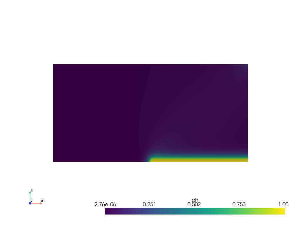
Plot: phase-field \(\phi\)

The phase-field result saved in the .vtu file is shown. For this, the file is loaded using PyVista.

file_vtu = pv.read(os.path.join(Data.results_folder_name, "paraview-solutions_vtu", "phasefieldx_p0_000149.vtu"))

file_vtu.plot(scalars='phi', cpos='xy', show_scalar_bar=True, show_edges=False)

Static Scene

Interactive Scene

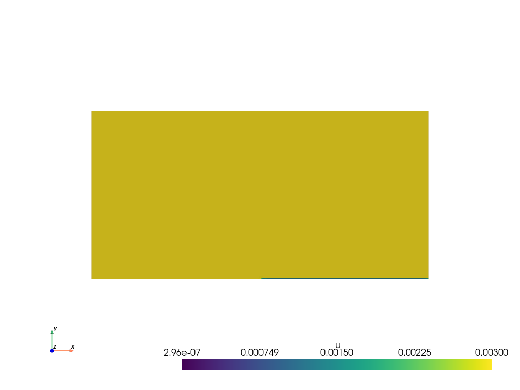
Plot: displacement \(\boldsymbol u\)

The displacements results saved in the .vtu file are shown. For this, the file is loaded using PyVista.

file_vtu = pv.read(os.path.join(Data.results_folder_name, "paraview-solutions_vtu", "phasefieldx_p0_000149.vtu"))
file_vtu.plot(scalars='u', cpos='xy', show_scalar_bar=True, show_edges=False)

Static Scene

Interactive Scene

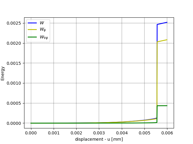
Plot: Displacement vs Fracture Energy

The vertical displacement is saved in S.dof_files[“top.dof”][“Uy”]. (Note: This simulation considers half of the model due to symmetry, so the results are multiplied by 2.)

displacement = 2 * S.dof_files["top.dof"]["Uy"]

fig, energyW = plt.subplots()

energyW.plot(displacement, 2 * S.energy_files['total.energy']["W"], 'b-', linewidth=2.0, label=r'$W$')
energyW.plot(displacement, 2 * S.energy_files['total.energy']["W_phi"], 'y-', linewidth=2.0, label=r'$W_{\phi}$')
energyW.plot(displacement, 2 * S.energy_files['total.energy']["W_gradphi"], 'g-', linewidth=2.0, label=r'$W_{\nabla \phi}$')

energyW.grid(color='k', linestyle='-', linewidth=0.3)
energyW.set_xlabel('displacement - u $[mm]$')
energyW.set_ylabel('Energy')
energyW.legend()

<matplotlib.legend.Legend object at 0x73426e598880>

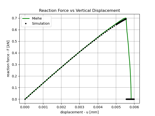
Plot: Force vs Vertical Displacement

Miehe = np.loadtxt(os.path.join("reference_solutions", "miehe_solution.csv"))

fig, ax_reaction = plt.subplots()

ax_reaction.plot(Miehe[:, 0], Miehe[:, 1], 'g-', linewidth=2.0, label='Miehe')
ax_reaction.plot(displacement, -S.reaction_files['bottom.reaction']["Ry"], 'k.', linewidth=2.0, label=S.label)

ax_reaction.grid(color='k', linestyle='-', linewidth=0.3)
ax_reaction.set_xlabel('displacement - u $[mm]$')
ax_reaction.set_ylabel('reaction force - F $[kN]$')
ax_reaction.set_title('Reaction Force vs Vertical Displacement')
ax_reaction.legend()

<matplotlib.legend.Legend object at 0x73426e79eb30>

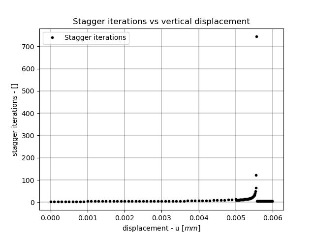
Plot: Staggered Iterations vs Vertical Displacement

fig, ax_convergence = plt.subplots()

ax_convergence.plot(displacement, S.convergence_files["phasefieldx.conv"]["stagger"], 'k.', linewidth=2.0, label='Stagger iterations')

ax_convergence.grid(color='k', linestyle='-', linewidth=0.3)
ax_convergence.set_xlabel('displacement - u $[mm]$')
ax_convergence.set_ylabel('stagger iterations - []')
ax_convergence.set_title('Stagger iterations vs vertical displacement')
ax_convergence.legend()

plt.show()