Force control

This script simulates a linear elastic problem using a force-control approach, based on the theory outlined in (Elasticity).

Model Overview

The model represents a square plate with:

• A fully fixed bottom edge, preventing both displacement and rotation.

• A controlled vertical force applied along the top edge.

The geometry, boundary conditions, and mesh structure are shown below. The plate is discretized using quadrilateral finite elements, suitable for 2D structural analysis.

#           F/\/\/\/\/\/\
#            ||||||||||||
#            *----------*
#            |          |
#            |          |
#            |          |
#            |          |
#            |          |
#            *----------*
#            /_\/_\/_\/_\
#     |Y    /////////////
#     |
#      ---X
#  Z /

Material Properties

The material properties are summarized in the table below:

	VALUE	UNITS
E	210	kN/mm2
nu	0.3	[-]

Import necessary libraries

import numpy as np
import matplotlib.pyplot as plt
import pyvista as pv
import dolfinx
import mpi4py
import petsc4py
import os

Import from phasefieldx package

from phasefieldx.Element.Elasticity.Input import Input
from phasefieldx.Element.Elasticity.solver.solver import solve
from phasefieldx.Boundary.boundary_conditions import bc_xy, get_ds_bound_from_marker
from phasefieldx.Loading.loading_functions import loading_Txy
from phasefieldx.PostProcessing.ReferenceResult import AllResults

Define Simulation Parameters

Data is an input object containing essential parameters for simulation setup and result storage:

• E: Young’s modulus, set to 210 kN/mm².

• nu: Poisson’s ratio, set to 0.3.

• save_solution_xdmf and save_solution_vtu: Set to False and True, respectively, specifying the file format to save displacement results (.vtu here).

• results_folder_name: Name of the folder for saving results. If it exists,

it will be replaced with a new empty folder.

Data = Input(E=210.0,
             nu=0.3,
             save_solution_xdmf=False,
             save_solution_vtu=True,
             results_folder_name="1101_force_control")

Mesh Definition

The mesh is a structured grid with quadrilateral elements:

• divx, divy: Number of elements along the x and y axes (10 each).

• lx, ly: Physical domain dimensions in x and y (1.0 units each).

divx, divy = 10, 10
lx, ly = 1.0, 1.0
msh = dolfinx.mesh.create_rectangle(mpi4py.MPI.COMM_WORLD,
                                    [np.array([0, 0]),
                                     np.array([lx, ly])],
                                    [divx, divy],
                                    cell_type=dolfinx.mesh.CellType.quadrilateral)

Boundary Identification

Boundary conditions and forces are applied to specific regions of the domain:

• bottom: Identifies the \(y=0\) boundary.

• top: Identifies the \(y=ly\) boundary.

fdim is the dimension of boundary facets (1D for a 2D mesh).

def bottom(x):
    return np.isclose(x[1], 0)

def top(x):
    return np.isclose(x[1], ly)

fdim = msh.topology.dim - 1

Using the bottom and top functions, we locate the facets on the bottom and top sides of the mesh, where \(y = 0\) and \(y = ly\), respectively. The locate_entities_boundary function returns an array of facet indices representing these identified boundary entities.

bottom_facet_marker = dolfinx.mesh.locate_entities_boundary(msh, fdim, bottom)
top_facet_marker = dolfinx.mesh.locate_entities_boundary(msh, fdim, top)

The get_ds_bound_from_marker function generates a measure for applying boundary conditions specifically to the facets identified by top_facet_marker and bottom_facet_marker, respectively. This measure is then assigned to ds_bottom and ds_top.

ds_bottom = get_ds_bound_from_marker(bottom_facet_marker, msh, fdim)
ds_top = get_ds_bound_from_marker(top_facet_marker, msh, fdim)

ds_list is an array that stores boundary condition measures along with names for each boundary, simplifying result-saving processes. Each entry in ds_list is formatted as [ds_, “name”], where ds_ represents the boundary condition measure, and “name” is a label used for saving. Here, ds_bottom and ds_top are labeled as “bottom” and “top”, respectively, to ensure clarity when saving results.

ds_list = np.array([
                   [ds_bottom, "bottom"],
                   ])

Function Space Definition

Define function spaces for the displacement field using Lagrange elements of degree 1.

V_u = dolfinx.fem.functionspace(msh, ("Lagrange", 1, (msh.geometry.dim, )))

Boundary Conditions

Dirichlet boundary conditions are applied as follows:

• bc_bottom: Fixes x and y displacement to 0 on the bottom boundary.

bc_bottom = bc_xy(bottom_facet_marker, V_u, fdim)

The bcs_list_u variable is a list that stores all boundary conditions for the displacement field \(\boldsymbol u\). This list facilitates easy management of multiple boundary conditions and can be expanded if additional conditions are needed.

bcs_list_u = [bc_bottom]
bcs_list_u_names = ["bottom"]

def update_boundary_conditions(bcs, time):
    return 0, 0, 0

External Load Definition

Here, we define the external load to be applied to the top boundary (ds_top). T_top represents the external force applied in the y-direction.

T_top = loading_Txy(msh)

The load is added to the list of external loads, T_list_u, which will be updated incrementally in the update_loading function.

T_list_u = [[T_top, ds_top]
           ]
f = None

Function: update_loading

The update_loading function is responsible for incrementally applying an external load at each time step, achieving a force-controlled quasi-static loading. This function allows for gradual increase in force along the y-direction on a specific boundary facet, simulating controlled force application over time.

Parameters:

• T_list_u: List of tuples where each entry corresponds to a load applied to a specific boundary or facet of the mesh.

• time: Scalar representing the current time step in the analysis.

Inside the function:

• val is calculated as 0.1 * time, a linear function of time, which represents the gradual application of force in the y-direction. This scaling factor (0.1 in this case) can be adjusted to control the rate of force increase.

• The value val is assigned to the y-component of the external force field on the top boundary by setting T_list_u[0][0].value[1], where T_list_u[0][0] represents the load applied to the designated top boundary facet (ds_top).

Returns:

• A tuple (0, val, 0) where:

• The first element is zero, indicating no load in the x-direction.

• The second element is val, the calculated y-directional force.

• The third element is zero, as this is a 2D example without z-component loading.

This function supports force-controlled quasi-static analysis by adjusting the applied load over time, ensuring a controlled force increase in the simulation.

def update_loading(T_list_u, time):
    val = 0.1 * time
    T_list_u[0][0].value[1] = petsc4py.PETSc.ScalarType(val)
    return 0, val, 0

f = None

Solver Call for a Static Linear Problem

We define the parameters for a simple, static linear boundary value problem with a final time t = 10.0 and a time step Δt = 1.0. Although this setup includes time parameters, they are primarily used for structural consistency with a generic solver function and do not affect the result, as the problem is linear and time-independent.

Parameters:

• final_time: The end time for the simulation, set to 10.0.

• dt: The time step for the simulation, set to 1.0. In a static context, this only provides uniformity with dynamic cases but does not change the results.

• path: Optional path for saving results; set to None here to use the default.

• quadrature_degree: Defines the accuracy of numerical integration; set to 2 for this problem.

Function Call: The solve function is called with:

• Data: Simulation data and parameters.

• msh: Mesh of the domain.

• V_u: Function space for \(\boldsymbol u\).

• bcs_list_u: List of boundary conditions.

• update_boundary_conditions, update_loading: update the boundary condition for the quasi static analysis

• ds_list: Boundary measures for integration on specified boundaries.

• dt and final_time to define the static solution time window.

final_time = 11.0
dt = 1.0

solve(Data,
      msh,
      final_time,
      V_u,
      bcs_list_u,
      update_boundary_conditions,
      f,
      T_list_u,
      update_loading,
      ds_list,
      dt,
      path=None,
      quadrature_degree=2,
      bcs_list_u_names=bcs_list_u_names)

All specified files deleted successfully.
All specified folders and their contents deleted successfully.
All specified folders and their contents deleted successfully.

Load results

Once the simulation finishes, the results are loaded from the results folder. The AllResults class takes the folder path as an argument and stores all the results, including logs, energy, convergence, and DOF files. Note that it is possible to load results from other results folders to compare results. It is also possible to define a custom label and color to automate plot labels.

S = AllResults(Data.results_folder_name)
S.set_label('Simulation')
S.set_color('b')

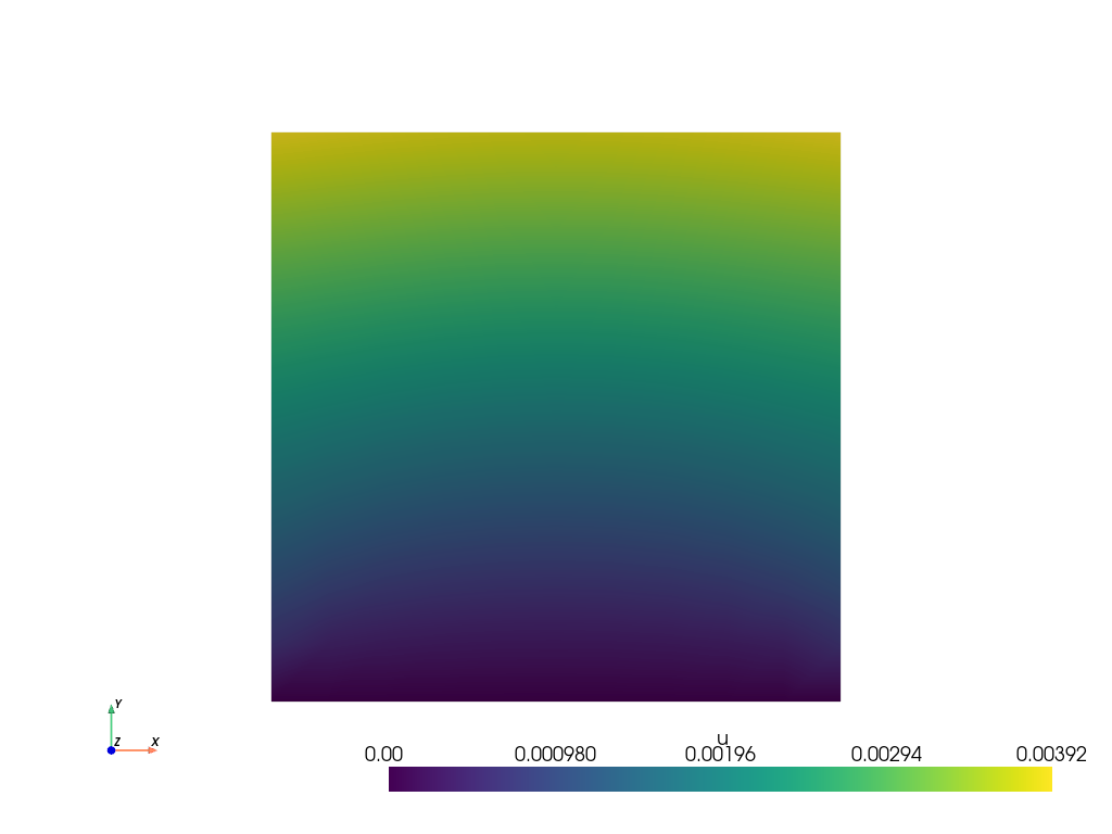
Plot: displacement \(\boldsymbol u\)

The displacement result saved in the .vtu file is shown. For this, the file is loaded using PyVista.

file_vtu = pv.read(os.path.join(Data.results_folder_name, "paraview-solutions_vtu", "phasefieldx_p0_000009.vtu"))
file_vtu.plot(scalars='u', cpos='xy', show_scalar_bar=True, show_edges=False)

Static Scene

Interactive Scene

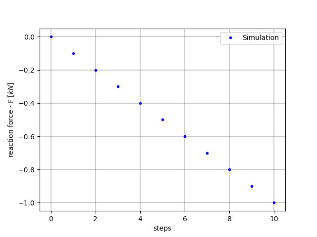
Steps vs. Reaction Force

Plot the steps versus the reaction force.

steps = S.dof_files["top.dof"]["#step"]

Plot steps vs reaction force

fig, ax = plt.subplots()

ax.plot(steps, S.reaction_files['bottom.reaction']["Ry"], S.color + '.', linewidth=2.0, label=S.label)

ax.grid(color='k', linestyle='-', linewidth=0.3)
ax.set_xlabel('steps')
ax.set_ylabel('reaction force - F $[kN]$')
ax.legend()

plt.show()